Spending becomes income and repeated domestic re-spending creates a multiplier effect.
Must know
- Injections are I G and X.
- Withdrawals are S T and M.
- The multiplier is the inverse of the total marginal withdrawal rate under the stated model.
Must know definitions
Circular flow of income: the flow of money between households and firms in an economy.
Income: a flow — money earned over a period of time.
Wealth: a stock measured at a point in time; net wealth is the value of assets minus liabilities.
Injections: additions to the circular flow of income (investment, I; government spending, G; exports, X).
Withdrawals (leakages): outflows from the circular flow of income (savings, S; taxation, T; imports, M).
Equilibrium national income: the level of national income at which planned AD equals planned AS (equivalently, injections equal withdrawals).
The multiplier: the ratio of the change in equilibrium real national income to the autonomous injection that caused it.
Marginal propensity to consume (MPC): the proportion of an additional unit of income spent on consumption.
Marginal propensity to save (MPS): the proportion of an additional unit of income saved.
Marginal propensity to tax (MPT): the proportion of an additional unit of income paid in tax.
Marginal propensity to import (MPM): the proportion of an additional unit of income spent on imports.
Marginal propensity to withdraw (MPW): the total proportion of an additional unit of income withdrawn from the circular flow (MPS + MPT + MPM).
The accelerator effect: changes in demand or output growth influence induced investment in additional capacity, subject to expectations and existing spare capacity.
Must know relationship: k = 1 / (MPS + MPT + MPM); ΔY = k × Δinjection under the stated model.
Symbols: k is the multiplier and ΔY is the income change. MPS, MPT and MPM are the fractions of additional income withdrawn as saving, tax and imports; enter 20% as 0.20. The multiplier has no unit; ΔY uses the same money units as the initial injection. The simple real-output result assumes spare capacity and stable propensities.
Explain and apply
Mechanism in brief: An injection becomes income for its recipients. Their additional consumption generates further income, while saving, tax and imports remove part from each round, making successive rounds smaller.
Distinguish: Do not double-count imported consumption; the initial injection is not the total income change.
Use the extract: Identify the initial injection and the proportions saved, taxed and spent on imports; distinguish the first round from the total effect.
The circular flow of income
- The circular flow of income shows the flow of money between households and firms in an economy.
- Households supply factors of production (land, labour, capital, enterprise) to firms and receive income in return (wages, rent, interest, profit).
- Households then spend this income on the goods and services firms produce.
- Saving, taxation and imports divert income from spending on domestic goods; investment, government spending and exports add demand for domestic output.
Figure 2.21 Circular flow of income
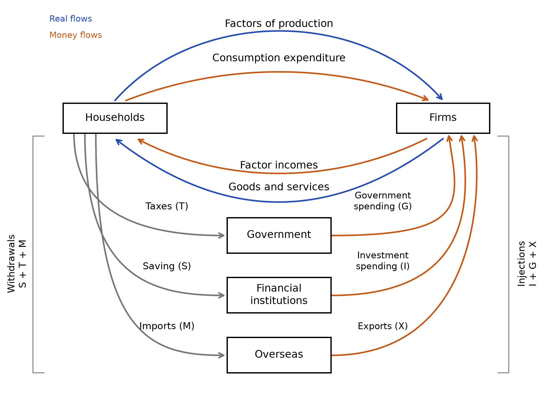
Read the diagram: Households supply factors and receive income; consumption spending pays firms for goods and services. Grey arrows show withdrawals; orange arrows from the other sectors show injections. S, T, I and G can exist in a closed economy; adding imports (M) and exports (X) makes it open. The sector links are simplified: each withdrawal need not equal its paired injection.
Income and wealth
- Income is a flow concept — money earned over a period of time (e.g. wages per month, interest per year).
- Wealth is a stock concept — the value of assets accumulated at a point in time (e.g. property, savings, shares).
- Income can build wealth, but only if some of it is saved rather than spent.
- Converting income into wealth means an individual must forego current consumption to enjoy greater welfare in future, so the opportunity cost of increased future wealth is current consumption foregone.
| Income | Wealth | |
|---|---|---|
| Nature | Flow (earned over a period) | Stock (accumulated at a point in time) |
| Examples | Wages, rent, dividends, interest | Property, savings, shares, physical assets |
| Key exam point | Measured per period (£ per month/year) | Measured at a moment in time; income saved over time builds wealth |
Injections and withdrawals
Injections are additions to the circular flow of income
investment (I), government spending (G), and exports (X).
Withdrawals (or leakages) are outflows from the circular flow
savings (S), taxation (T), and imports (M).
Injections have a multiplier effect on national income, expanding it; withdrawals have the opposite effect, causing a multiplied contraction of national income.
| Injections (add to circular flow) | Withdrawals (leak from circular flow) |
|---|---|
| Investment (I) | Savings (S) |
| Government spending (G) | Taxes (T) |
| Exports (X) | Imports (M) |
The impact of net injections and net withdrawals
Planned injections exceed withdrawals → spending and income tend to rise.
Planned withdrawals exceed injections → spending and income tend to fall.
Planned injections equal withdrawals → equilibrium income. These are three alternative cases.
- Be able to analyse real-world changes in terms of their net effect on the circular flow.
For example
A higher interest rate may discourage investment and encourage saving → planned spending falls relative to income → firms reduce output if demand weakens. This does not imply that the money stock must fall.
Equilibrium level of real national output
- Equilibrium national income occurs where planned aggregate demand equals planned aggregate supply — equivalently, where injections equal withdrawals.
- Any factor that shifts AD or AS will change this equilibrium; the resulting change in the price level and real output depends on the shape of the AS curve at the point of intersection (covered in detail in AD/AS equilibrium).
The multiplier and multiplier process
- The multiplier is the ratio of the change in equilibrium real national income to the autonomous change (the injection) that caused it.
- For example, if a £1m injection into the circular flow leads to a £2m increase in national income, the multiplier = 2.
→ Government injects £100m (↑ G) → this becomes income for workers and suppliers → they spend a proportion of it (determined by the MPC) on domestic goods and services → this spending becomes income for others, who spend a proportion of that → and so on in successive rounds → each round is smaller than the last because some income leaks out as savings, tax, and imports → total increase in national income = initial injection × multiplier
When injections fall, the process works in reverse
a withdrawal from the circular flow causes a multiplied contraction of national income.
Marginal propensities and their effects on the multiplier
| Term | Definition | Formula | Effect on multiplier |
|---|---|---|---|
| Marginal propensity to consume (MPC) | Proportion of an extra £1 of income spent on consumption | ΔC / ΔY | ↑ MPC → ↑ multiplier |
| Marginal propensity to save (MPS) | Proportion of an extra £1 of income saved | ΔS / ΔY | ↑ MPS → ↓ multiplier |
| Marginal propensity to tax (MPT) | Proportion of an extra £1 of income paid in tax | ΔT / ΔY | ↑ MPT → ↓ multiplier |
| Marginal propensity to import (MPM) | Proportion of an extra £1 of income spent on imports | ΔM / ΔY | ↑ MPM → ↓ multiplier |
| Marginal propensity to withdraw (MPW) | Total proportion of an extra £1 of income withdrawn from the circular flow | MPS + MPT + MPM | ↑ MPW → ↓ multiplier |
- The higher the MPC, the higher the multiplier, since more of each round of income is re-spent domestically rather than leaking out.
- Conversely, the multiplier depends inversely on the size of withdrawals: the higher the MPW, the smaller the multiplier.
- In a simple two-sector economy with no tax or trade, MPC + MPS = 1. With taxes and imports, use the stated withdrawal propensities consistently. If MPC means total consumption rather than domestic re-spending, adding MPM to it as another use of income double-counts imported consumption.
Calculating the multiplier
| Formula | When to use | Logic |
|---|---|---|
| Multiplier = 1 / (1 − MPC) | Simple two-sector economy (savings is the only leakage) | 1/(1-MPC) sums the infinite geometric series of successive spending rounds |
| Multiplier = 1 / MPW | Full economy, where MPW = MPS + MPT + MPM | The multiplier is inversely proportional to the total withdrawal rate |
if MPS = 0.15, MPT = 0.20 and MPM = 0.05:
MPW = MPS + MPT + MPM = 0.15 + 0.20 + 0.05 = 0.40. In this example, 0.60 of an extra unit of income is re-spent on domestic output.
Multiplier = 1 / MPW = 1 / 0.4 = 2.5
A £100m injection → total increase in national income of £100m × 2.5 = £250m
The significance of the multiplier for shifts in AD
- If the multiplier is 3, an increase in government expenditure causes a larger rightward shift in AD than if the multiplier is only 2 — and correspondingly, a greater impact on economic activity, output, and employment.
| Multiplier value | Initial injection | Total shift in AD |
|---|---|---|
| 2 | £10bn | £20bn |
| 3 | £10bn | £30bn |
| 4 | £10bn | £40bn |
→ Higher multiplier → same-sized injection produces a larger increase in AD and economic activity → more powerful (and more inflationary, if AS is inelastic) demand-side policy
The multiplier also works in reverse
a withdrawal (e.g. ↓ G, or ↑ interest rates raising savings) causes a multiplied fall in AD, so austerity or contractionary policy can have a larger negative effect on the economy than the initial change alone.
Do not apply 1/(1-MPC) when MPT and MPM are given in the question — use 1/MPW instead, since 1/(1-MPC) only holds in a simple two-sector economy with no tax or trade.
A common exam evaluation point
the multiplier may be smaller in practice than the formula suggests if:
households have a high MPM (an open economy with heavy import dependence, so much of the extra spending leaks abroad)
consumer confidence is low (households save rather than spend, raising MPS)
the economy has little spare capacity (so an AD increase pushes up the price level rather than raising real output, weakening the real multiplier effect)
The full multiplier effect also takes time to work through the economy, so the short-run impact may be smaller than the theoretical value implies.
The accelerator effect
- The accelerator effect links induced investment to changes in demand or output. In the simple model, a faster increase in output requires a larger addition to the capital stock; replacement investment is a separate component.
- When firms expect demand to grow faster, they may invest in additional capacity. If demand is still growing but more slowly, less new capacity may be needed, so induced investment can fall. Existing spare capacity and expectations affect the response.
Expansion: faster expected demand growth → firms may add capacity → investment rises → AD increases. Slowdown: weaker expected demand growth → less new capacity is needed → investment may fall even while GDP is still growing. The response depends on spare capacity and expectations.
- This explains why investment is the most volatile component of AD, and why investment-led downturns can be severe.
- Combined with the multiplier, this produces the multiplier-accelerator model of the business cycle: an initial rise in demand triggers multiplied income growth, which triggers accelerator-driven investment, which further boosts AD — amplifying both booms and busts.
A high calculated multiplier does not guarantee a large real-output gain. Capacity constraints can raise prices, and actual leakages or delays can reduce the effect; distinguish the model's total-income result from the real response.
Rapid recap
Flows: households supply factors and receive income; firms receive consumption spending and supply output. S, T and M are withdrawals; I, G and X are injections.
Adjustment: injections above withdrawals tend to raise income; rising income generates further withdrawals. Equilibrium requires total injections = total withdrawals, not equality of each paired flow.
Calculate: k = 1/MPW; ΔY = k × the initial autonomous spending injection. Use decimal propensities and distinguish the initial change from the total effect.
Judge: leakages reduce the multiplier; supply constraints may turn extra spending into prices rather than real output.
Diagram cue: reconstruct circular-flow directions, injections and withdrawals.
Related chapters: Unit 2 chapter 2 (p. 32) · Unit 2 chapter 7 (p. 77)