Aggregate demand is total planned spending on domestically produced output.
Must know
- AD equals C plus I plus G plus X minus M.
- A price-level change causes movement along AD.
- Changes in spending determinants shift AD.
Must know definitions
Aggregate demand (AD) — the total demand for all final goods and services in an economy at a given price level over a period of time.
Consumption (C) — household spending on goods and services.
Investment (I) — spending by firms on capital goods that will be used to produce goods and services in the future.
Gross investment — total spending on capital goods before depreciation is accounted for.
Net investment — gross investment minus depreciation.
Government spending (G) — spending by central and local government on goods and services; excludes transfer payments.
Transfer payments — government payments to individuals without any goods or services provided in return (e.g. pensions, unemployment benefits); not included in G.
Net exports (X − M) — the value of exports minus the value of imports.
Disposable income — income remaining after direct taxes have been paid and transfer payments received.
Savings — the part of disposable income that is not spent on consumption.
Savings ratio — the percentage of disposable income that is saved.
Animal spirits — Keynes' term for the confidence, optimism, and risk appetite of entrepreneurs that drives investment decisions.
Paradox of thrift — the observation that if all households increase savings simultaneously, the fall in consumption may reduce AD and incomes so much that total savings actually fall.
Must know relationship: AD = C + I + G + (X − M).
Symbols: C = consumption; I = investment; G = government purchases; X = exports; M = imports. Use values in the same currency and period. Transfers are not directly part of G, and imports are deducted to isolate domestic output.
Explain and apply
Mechanism in brief: Lower interest rates reduce some borrowing costs and saving returns, potentially raising consumption and investment. These changes raise planned domestic spending and shift AD right; import leakage can weaken the domestic effect.
Distinguish: Transfers affect disposable income rather than entering G directly; imports are subtracted to isolate domestic production.
Use the extract: Identify the spending component that changes and the evidence for its response; explain how this affects total planned spending.
Aggregate demand (AD) — the total demand for all final goods and services in an economy at a given price level over a period of time, calculated as AD = C + I + G + (X − M).
The AD formula and its components
| Component | Definition | Illustrative share of AD | Key driver |
|---|---|---|---|
| Consumption (C) | Household spending on goods and services | 60% | Disposable income |
| Investment (I) | Spending by firms on capital goods (machinery, buildings, technology) | 18% | Interest rates, business confidence |
| Government spending (G) | Spending by central and local government on goods and services | 20% | Fiscal policy, economic cycle |
| Net exports (X − M) | Exports minus imports | 2% | Exchange rate, world income, competitiveness |
Exam tip: The shares above are a hypothetical economy, not current UK data. Here consumption is the largest component, so a 1% increase in C adds more to expenditure than a 1% increase in I or G, holding everything else unchanged. Net exports can be negative or close to zero, making percentage comparisons misleading. These are initial expenditure effects, not a prediction of the final change in real GDP.
- Useful application: compare the size of each AD component and its likely change in the given economy before judging which has the greatest effect.
Transfer payments — government payments to individuals without any goods or services being provided in return (e.g. pensions, unemployment benefits).
- These are NOT included in G because they do not represent production of new output — they merely redistribute income.
The AD curve
Figure 2.6 Movement along AD
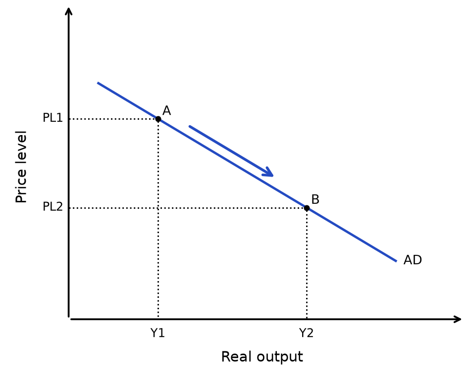
Read the diagram: The price level changes, holding other influences fixed. The arrow shows movement from A to B along the same AD curve. Real output is labelled Y and the price level PL; this is not a shift of the curve.
Why the AD curve slopes downward
| Reason | Mechanism | Condition |
|---|---|---|
| Real balance effect (wealth effect) | ↑ PL → purchasing power of money balances falls → households and firms can buy fewer goods/services with the same nominal income → real output demanded falls | Assumes nominal money holdings do not rise with prices. |
| International competitiveness effect | ↑ PL → domestic goods relatively more expensive than foreign goods → exports fall, imports rise → net trade (X − M) falls → real output demanded falls | Depends on relative prices, exchange rates and trade responsiveness. |
| Interest rate effect | ↑ PL → households and firms need more money for transactions → ↑ demand for money → ↑ interest rates → ↓ borrowing and spending → ↓ C and I → ↓ real output demanded | Depends on monetary conditions and interest-sensitive spending. |
Movement along vs shift of AD
| Change | Cause | Effect on diagram |
|---|---|---|
| Movement along AD | Change in the price level | Expansion (↑ PL to ↓ PL) or contraction (↓ PL to ↑ PL) along the existing curve |
| Shift of AD | Change in any component (C, I, G, X − M) | Entire curve shifts right (↑ AD) or left (↓ AD) |
→ Change in PL → movement along the AD curve
→ Change in C, I, G, or (X − M) at every PL → shift of the entire AD curve
Figure 2.7 Shifts of AD — Increase
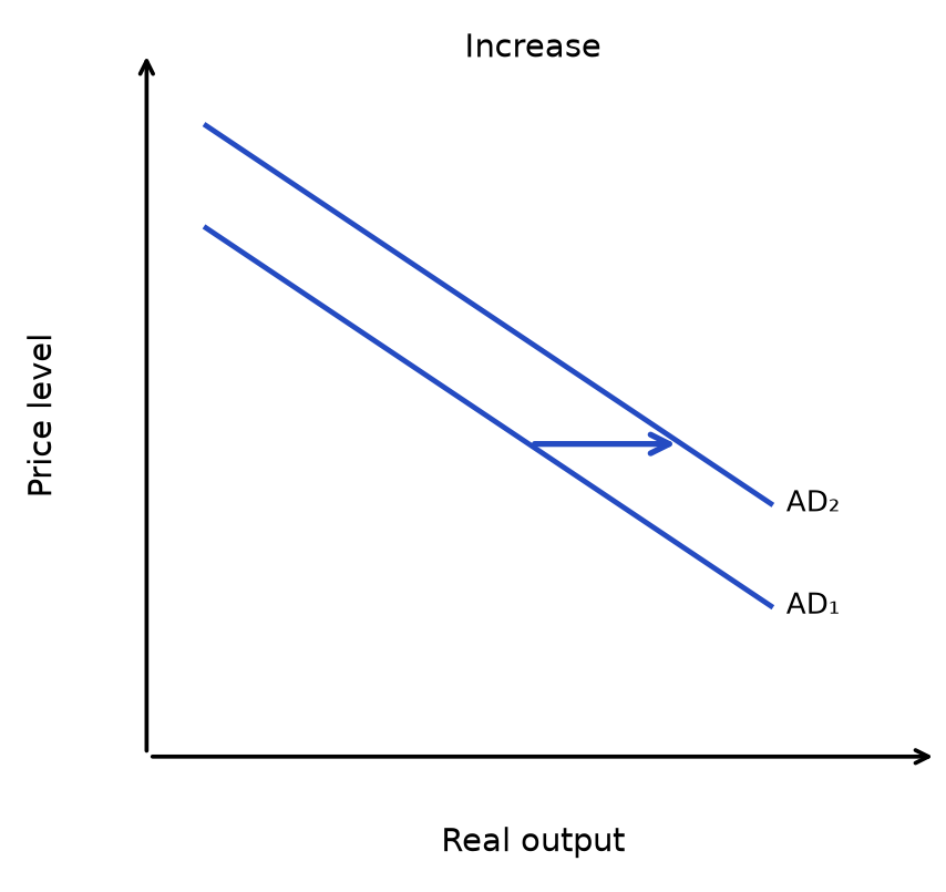
Figure 2.8 Shifts of AD — Decrease
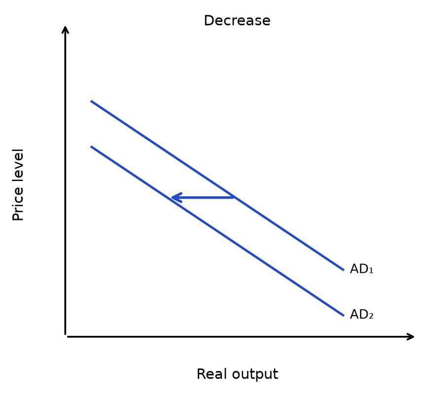
Read the diagram: Each panel shows a change in a non-price determinant, holding other influences fixed. The arrow runs from curve 1 to curve 2: an increase is a rightward shift; a decrease is a leftward shift. Compare quantities at the same vertical-axis value.
Common mistake: don't confuse a change in the price level (movement along the curve) with a change in one of AD's components (a shift of the whole curve) — only C, I, G, or (X − M) changes shift AD.
Consumption (C)
Consumption — household spending on goods and services.
- The largest component of AD.
Disposable income — income remaining after direct taxes have been paid and transfer payments (benefits) received.
- This is the amount households can choose to spend or save.
Influences on consumption
| Factor | Mechanism | Condition |
|---|---|---|
| Disposable income | ↑ income after tax + benefits → ↑ spending power → ↑ C → ↑ AD | Size depends on the marginal propensity to consume. |
| Interest rates | ↓ interest rates → ↓ reward from saving + ↓ cost of borrowing → ↑ spending on credit + ↑ C | Net savers may lose interest income; confidence also matters. |
| Consumer confidence | ↑ confidence about future income/job security → ↑ willingness to spend → ↑ C | Expectations may change before spending responds. |
| Wealth effect | ↑ house prices / share prices → households feel wealthier → ↑ spending out of wealth → ↑ C | Gains are unevenly distributed and may be illiquid. |
| Availability of credit | Banks more willing to lend → easier access to loans/credit cards → ↑ C | Borrowers must still qualify and be willing to borrow. |
| Government policy | ↓ direct tax → ↑ disposable income → ↑ C; ↑ welfare payments → ↑ disposable income for low-income groups → ↑ C | Some additional disposable income may be saved or spent on imports. |
Savings and the savings ratio
Savings — the part of disposable income that is not spent on consumption.
Savings ratio — the percentage of disposable income that is saved, calculated as (savings / disposable income) × 100.
Relationship between savings and consumption:
→ Income is either spent or saved → C + S = disposable income → ↑ savings ratio → ↓ proportion of income spent → ↓ C → ↓ AD (in the short run)
→ ↓ savings ratio → ↑ proportion of income spent → ↑ C → ↑ AD (in the short run)
Factors influencing the savings ratio
| Factor | Effect on savings ratio | Mechanism |
|---|---|---|
| Disposable income | ↑ income → ↑ ability to save → ↑ savings ratio | Higher-income households tend to save a larger proportion of income |
| Real interest rate on savings | ↑ interest rate → ↑ reward from saving → ↑ savings ratio | Higher return makes saving more attractive relative to spending |
| Consumer confidence | ↓ confidence (fear of unemployment) → ↑ precautionary saving → ↑ savings ratio | Households save more as a buffer against expected hardship |
| Tax incentives to save | ↑ tax-free savings accounts / ISAs → ↑ incentive to save → ↑ savings ratio | Tax relief increases the effective return on savings |
| Age structure of population | The effect depends on life-cycle stages: working households may save for retirement, while retired households may draw down accumulated assets. | Wealth is a stock; holding more wealth does not necessarily mean saving a larger share of current income. |
| Deposit requirements | ↑ required deposits for mortgages → households must save more to buy a house → ↑ savings ratio | Higher deposit thresholds force more saving, reduce C |
| Availability of savings institutions | ↑ access to banks/savings accounts → easier to save → ↑ savings ratio | In developing countries, lack of banking access limits saving |
| Cultural / social factors | Cultures that value frugality → ↑ savings ratio | Social norms around debt, saving, and consumption vary by country |
Effects of changes in the savings ratio
| Direction | Short-run effect | Long-run effect |
|---|---|---|
| ↓ savings ratio | Higher C can raise AD and real output with spare capacity; inflation and imports may rise. The current-account effect depends on other components. | Lower saving may limit investment financing in some settings, but credit conditions, foreign capital and expected demand also matter; lower investment is not automatic. |
| ↑ savings ratio | Lower C can reduce AD and income; inflationary pressure and imports may ease. Total realised saving may fail to rise as income falls. | Higher saving can support investment under suitable financing and demand conditions. It does not automatically lower interest rates or raise investment. The paradox of thrift concerns the fall in income frustrating intended saving. |
Exam evaluation — the paradox of thrift:
→ If everyone saves more simultaneously → ↓ C → ↓ AD → ↓ economic growth → ↓ incomes → people end up saving less than they intended because their income has fallen → individual rationality leads to collective harm — this is Keynes' paradox of thrift
Investment (I)
Investment — spending by firms on capital goods (machinery, buildings, technology) that will be used to produce goods and services in the future.
Gross investment — total spending on capital goods before depreciation is accounted for.
Net investment — gross investment minus depreciation (the wear and tear on existing capital).
- Net investment = gross investment − depreciation.
- If net investment is positive, the economy's capital stock is growing.
Influences on investment
| Factor | Mechanism | Condition |
|---|---|---|
| Interest rates | ↓ interest rates → ↓ cost of borrowing → more investment projects become profitable → ↑ I | Weak expected demand may outweigh cheaper borrowing. |
| Business confidence / animal spirits | ↑ confidence about future demand → firms expect higher returns → ↑ willingness to invest → ↑ I | Expectations can reverse; uncertainty may delay projects. |
| Economic growth rate | ↑ GDP → ↑ consumer spending → ↑ firm revenue and profits → ↑ retained profits available for investment → ↑ I | Spare capacity may reduce the need to expand production. |
| Access to credit | Banks willing to lend → firms can borrow to invest → ↑ I; credit crunch → banks refuse loans → ↓ I | Access alone is insufficient if expected returns are low. |
| Corporation tax | ↓ corporation tax → firms keep more profit → ↑ funds available for investment → ↑ I | Retained profits may be saved or distributed instead. |
| Government subsidies / tax relief | Government provides investment allowances or subsidies → ↓ effective cost of investment → ↑ I | Additional investment depends on eligibility and whether firms would invest anyway. |
Animal spirits (Keynes): Keynes argued that investment is driven not only by rational calculation but also by "animal spirits" — the confidence, optimism, and risk appetite of entrepreneurs.
- When animal spirits are strong → ↑ I → AD maintained.
- When animal spirits are weak (uncertainty, pessimism) → ↓ I → ↓ AD → economy may lapse into recession.
Government policy to promote investment
→ ↓ corporation tax → ↑ retained profits → ↑ I
→ Tax relief on investment (capital allowances) → ↓ effective cost of investment → ↑ I
→ Subsidies for research and development (R&D) → ↑ incentive to invest in innovation → ↑ I
Government spending (G)
Government spending (G) — spending by central and local government on goods and services (e.g. education, healthcare, defence, infrastructure).
- Excludes transfer payments.
Influences on government spending
| Factor | Mechanism | Condition |
|---|---|---|
| Fiscal policy (discretionary) | Government chooses to change G to manage the economy → expansionary: ↑ G to ↑ AD during recession; contractionary: ↓ G to ↓ AD during boom | Multiplier size and spare capacity affect the output response. |
| Economic cycle (automatic stabilisers) | During a recession, benefit payments rise automatically and support disposable income and consumption. They are transfers, not G in the AD identity. | Transfers support C; they are not purchases counted in G. |
| Market failure correction | Government may ↑ G to provide public goods (defence, street lighting) and merit goods (education, healthcare) that the free market under-provides | Welfare gains depend on targeting and delivery. |
| Political priorities | Government may ↑ G before elections to gain favour, or ↓ G to reduce budget deficit as part of austerity | The deficit also depends on tax receipts and the economic response. |
Net exports (X − M)
Net exports — the value of exports minus the value of imports (X − M).
- A positive value means a trade surplus; a negative value means a trade deficit.
Influences on net trade balance
Real income (domestic)
Mechanism: ↑ domestic GDP → ↑ disposable income → ↑ spending on imports (imports are normal goods) → ↑ M → ↓ (X − M)
Arrow chain: ↑ domestic income → ↑ M → ↓ net exports → ↓ AD
Exchange rate
Mechanism: ↓ exchange rate (depreciation) → exports cheaper for foreign buyers, imports dearer for domestic buyers → ↑ X, ↓ M → ↑ (X − M) → ↑ AD; BUT depends on PED of exports/imports
Arrow chain: ↓ exchange rate → ↑ X (if demand is elastic), ↓ M → ↑ (X − M) → ↑ AD
World economic growth
Mechanism: ↑ GDP of trading partners → ↑ demand for exports → ↑ X → ↑ (X − M) → ↑ AD
Arrow chain: ↑ world income → ↑ demand for exports → ↑ X → ↑ AD
International competitiveness
Mechanism: ↓ domestic inflation relative to trading partners → domestic goods cheaper → ↑ X, ↓ M → ↑ (X − M)
Arrow chain: ↓ relative inflation → ↑ competitiveness → ↑ X, ↓ M → ↑ AD
Protectionism
Mechanism: ↑ tariffs/quotas by trading partners → ↓ X; ↑ domestic protectionism → ↓ M but may trigger retaliation → ↓ X
Arrow chain: ↑ foreign tariffs → ↓ X → ↓ AD; retaliation may offset ↓ M
Non-price factors (quality, innovation, trade deals)
Mechanism: ↑ product quality / innovation / trade bloc membership → foreign buyers prefer domestic goods → ↑ X
Arrow chain: ↑ quality / innovation → ↑ X → ↑ (X − M) → ↑ AD
Common mistake: don't assume a depreciation always improves the trade balance — check the Marshall-Lerner condition below before concluding.
Exchange rate effect — the Marshall-Lerner condition (exam evaluation):
→ Depreciation can make exports cheaper in foreign currency and imports dearer in domestic currency → under the standard Marshall–Lerner assumptions, including initially balanced trade and full price pass-through, the trade balance improves if |PED_X| + |PED_M| > 1.
→ In the short run, contracts and inelastic demand may limit volume changes → measured in domestic currency, the import bill may rise before export receipts increase enough to offset it. Export receipts do not necessarily fall simply because the foreign-currency export price falls. A J-curve occurs if an initial deterioration is followed by improvement as volumes adjust sufficiently.
Summary: factors that shift AD
- Quick exam reference — memorise these triggers for data response questions:
| Component | Factors that ↑ AD (shift right) | Factors that ↓ AD (shift left) |
|---|---|---|
| C (Consumption) | ↓ interest rates, ↑ disposable income, ↑ consumer confidence, ↑ house prices (wealth effect), ↑ credit availability | ↑ interest rates, ↓ disposable income, ↓ confidence, ↓ house prices, ↓ credit availability |
| I (Investment) | ↓ interest rates, ↑ business confidence (animal spirits), ↑ economic growth, ↓ corporation tax, ↑ access to credit | ↑ interest rates, ↓ confidence, ↑ corporation tax, credit crunch |
| G (Government spending) | Higher government purchases (expansionary fiscal policy). Transfers support C rather than entering G. | ↓ G (austerity, contractionary fiscal policy) |
| X − M (Net exports) | ↓ exchange rate (if PED elastic), ↑ world GDP, ↑ competitiveness, ↑ trade deals | ↑ exchange rate, ↓ world GDP (global recession), ↑ foreign protectionism, ↓ competitiveness |
Exam explanation stems: aggregate demand
Use these ready-made stems to explain AD in exam answers:
AD shift via consumption
Lower borrowing costs and saving returns may raise C and I → AD shifts right. The effect depends on each component’s initial size, the scale of its change, confidence and leakages; the largest component need not make the largest contribution to a particular change.
AD shift via investment
↑ business confidence (animal spirits) → firms expect higher returns → ↑ I → AD shifts right. Note that investment also ↑ the capital stock → ↑ LRAS → ↑ long-run productive capacity (a supply-side benefit as well as a demand-side effect).
AD shift via net exports
Depreciation can make exports cheaper abroad and imports dearer domestically. If net export spending rises, AD shifts right. Under the standard Marshall–Lerner assumptions, |PEDx| + |PEDm| > 1 favours trade-balance improvement; contracts, pass-through and supply responses affect the timing.
Wealth effect
↑ house prices → households feel wealthier → ↑ spending out of housing wealth (equity withdrawal) → ↑ C → AD shifts right. Conversely, ↓ house prices → negative wealth effect → ↓ C → AD shifts left.
Paradox of thrift for evaluation
If all households ↑ savings simultaneously → ↓ C → ↓ AD → ↓ economic growth → ↓ incomes → households end up saving less than intended → individual rationality leads to collective harm. Use this to evaluate the effect of an ↑ savings ratio.
Confidence and debt commitments determine whether households and firms respond. If spending rises mainly on imports, domestic output gains are smaller, so consider both the behavioural response and the destination of expenditure.
Rapid recap
Identify: AD = C + I + G + X − M. Name the component affected and explain why spending changes before drawing the shift.
Separate: government purchases enter G; transfers and income tax affect disposable income and C. Imports are deducted to exclude overseas production.
Judge: confidence, borrowing costs, saving and import leakage change the size of the domestic response. A rise in one component need not raise total AD if another falls sufficiently.
Diagram cue: show the justified AD shift and explain the affected spending component.
Related chapters: Unit 2 chapter 3 (p. 44) · Unit 2 chapter 4 (p. 55)
Why this connects: Investment is spending in current AD and can create capital that increases future LRAS. These effects use different mechanisms and may occur at different times.