AD and AS together determine the model's equilibrium price level and real output.
Must know
- Demand increases usually raise output and prices with upward-sloping SRAS.
- Supply increases usually raise output and lower prices.
- Spare capacity affects the balance between output and price changes.
Must know definitions
Equilibrium real national output — the level of output where planned aggregate demand equals planned aggregate supply.
Stagflation — inflation combined with stagnant or weak economic activity and high unemployment; an adverse supply shock can produce this combination.
Output gap — the difference between actual real output and potential (full-employment) real output; can be positive (economy overheating) or negative (spare capacity).
Explain and apply
Mechanism in brief: An increase in planned expenditure encourages firms to increase production. As spare capacity diminishes, rising costs and bottlenecks mean more of the adjustment occurs through prices rather than extra real output.
Distinguish: The vertical axis is the price level, not the inflation rate; simultaneous shifts require attention to relative size.
Use the extract: Locate spare capacity and identify whether the shock affects demand or supply before predicting output and the price level.
Equilibrium real national output — the level of output where planned aggregate demand equals planned aggregate supply (planned AD = planned AS).
This section bridges AD and AS
it shows how shifts in either curve determine the actual price level and real output in the economy.
It also shows why the shape of the AS curve (SRAS vs classical/Keynesian LRAS) fundamentally changes the outcome.
The AD/AS equilibrium diagram
Figure 2.14 AD and AS equilibrium
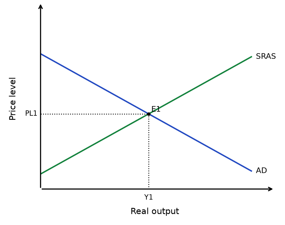
Read the diagram: At the intersection, planned aggregate demand equals aggregate supply. Read the two equilibrium coordinates from the axes. This is the short-run outcome with upward-sloping SRAS.
→ Equilibrium occurs where the AD curve intersects the AS curve → at this point, planned spending exactly matches planned output → no tendency for PL or Y to change (ceteris paribus)
Exam tip
Any change in AD or AS causes the economy to move to a new equilibrium — a new intersection point with a new PL and Y.
Always identify (1) which curve moved, (2) which direction, and (3) the resulting new equilibrium point before describing the effect.
Effects of AD shifts on equilibrium
- The spec requires you to draw AD/AS diagrams showing how shifts in AD affect both the equilibrium price level and equilibrium real output, ceteris paribus.
Figure 2.15 AD and AS equilibrium
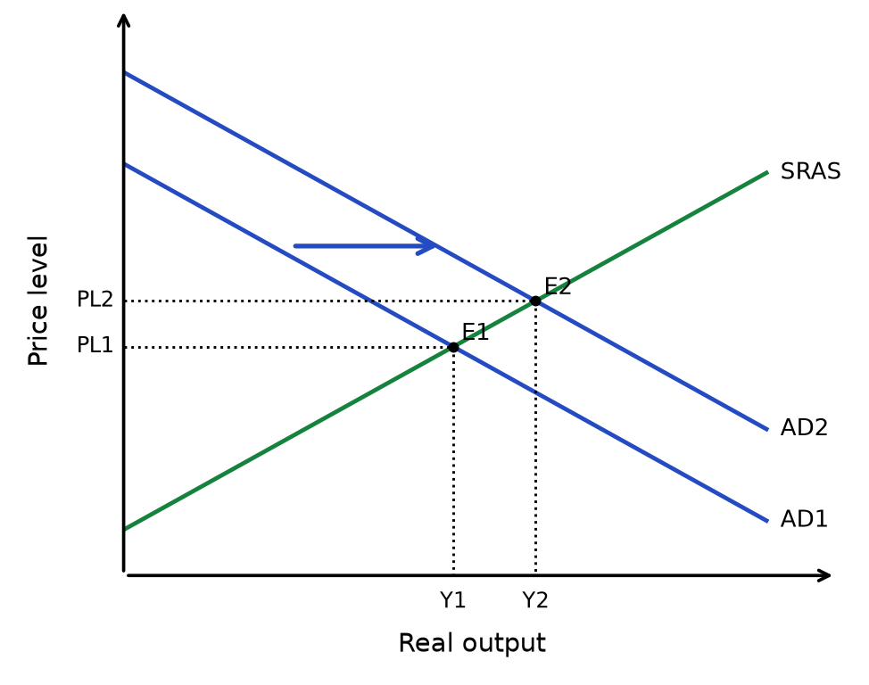
Read the diagram: Identify a non-price determinant that changes AD → shift AD right, holding the other curve fixed → find the new intersection → price level rises and real output rises. The price-level change is a movement along the unchanged curve. This result assumes upward-sloping SRAS; spare capacity and the curve’s slope determine the real-output response. A higher price level is not the same as a permanently higher inflation rate.
Figure 2.16 AD and AS equilibrium
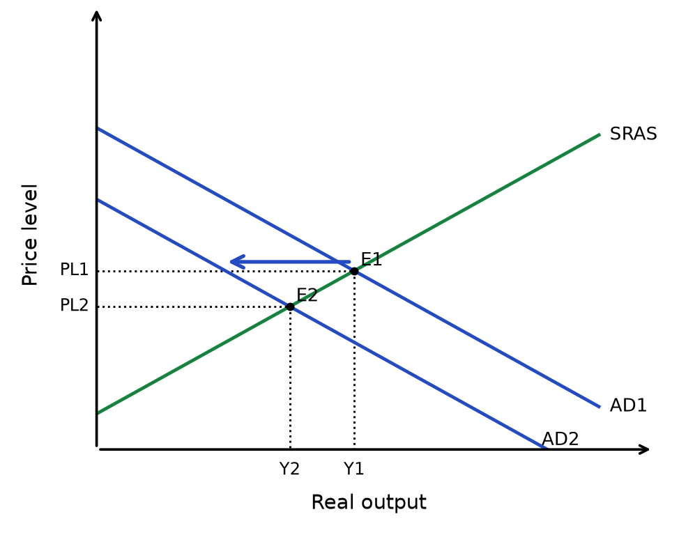
Read the diagram: Identify a non-price determinant that changes AD → shift AD left, holding the other curve fixed → find the new intersection → price level falls and real output falls. The price-level change is a movement along the unchanged curve. This result assumes upward-sloping SRAS; spare capacity and the curve’s slope determine the real-output response. A higher price level is not the same as a permanently higher inflation rate.
| AD shift | Effect on PL | Effect on real GDP | Example trigger |
|---|---|---|---|
| AD shifts right (↑ AD) | ↑ | ↑ | ↓ interest rates, ↑ C, ↑ G, ↓ exchange rate, ↑ business/consumer confidence |
| AD shifts left (↓ AD) | ↓ | ↓ | ↑ interest rates, ↓ confidence, ↓ G, ↑ exchange rate |
Worked chain (AD shift right)
→ ↓ interest rates → ↓ cost of borrowing → ↑ C and ↑ I → AD shifts right (AD1 to AD2) → at the original PL1, planned spending now exceeds planned output → firms respond by raising output AND prices (moving up along SRAS) → new equilibrium at (PL2, Y2), where PL2 > PL1 and Y2 > Y1
Effects of AS shifts on equilibrium
- A change in the conditions of supply shifts the AS curve itself (not caused by AD), producing the opposite PL/Y relationship to an AD shift.
Figure 2.17 AD and AS equilibrium
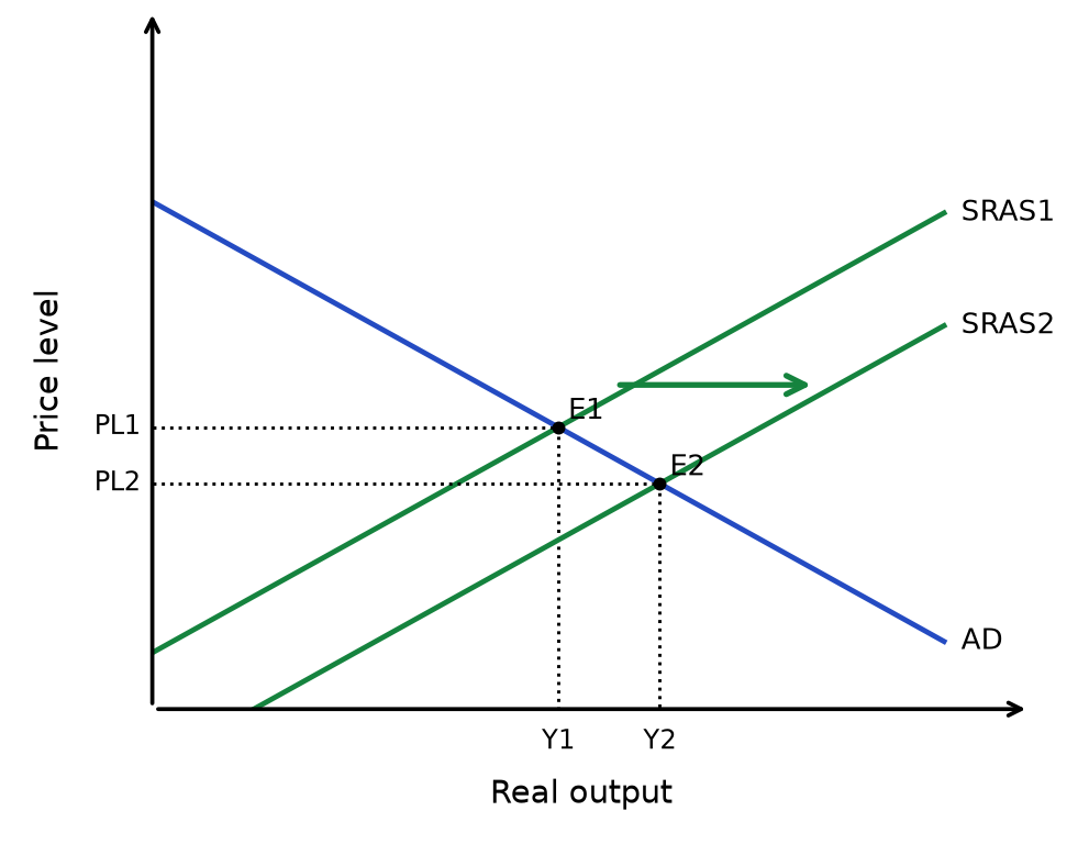
Read the diagram: Identify a non-price determinant that changes SRAS → shift SRAS right, holding the other curve fixed → find the new intersection → price level falls and real output rises. The price-level change is a movement along the unchanged curve. This result assumes upward-sloping SRAS; spare capacity and the curve’s slope determine the real-output response. A higher price level is not the same as a permanently higher inflation rate.
Figure 2.18 AD and AS equilibrium
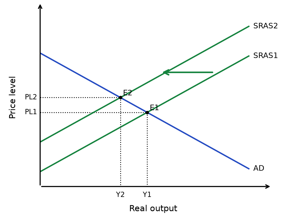
Read the diagram: Identify a non-price determinant that changes SRAS → shift SRAS left, holding the other curve fixed → find the new intersection → price level rises and real output falls. The price-level change is a movement along the unchanged curve. This result assumes upward-sloping SRAS; spare capacity and the curve’s slope determine the real-output response. A higher price level is not the same as a permanently higher inflation rate.
| AS shift | Effect on PL | Effect on real GDP | Example trigger |
|---|---|---|---|
| AS shifts right (↑ AS) | ↓ | ↑ | ↓ commodity/oil prices, ↑ productivity, ↓ wages, ↓ indirect tax, ↑ subsidies |
| AS shifts left (↓ AS) | ↑ | ↓ | ↑ commodity/oil prices, ↑ wages, ↓ exchange rate (dearer imports), ↑ indirect tax |
Exam tip — stagflation
A leftward shift in SRAS (e.g. from an oil price shock) is the classic cause of stagflation — rising prices combined with falling output.
This is the key diagram to distinguish demand-side inflation from cost-push (supply-side) inflation:
AD shifts right → PL and Y move in the SAME direction
SRAS shifts left → PL and Y move in OPPOSITE directions
Do not read every rightward curve shift the same way — an AD shift right and an AS shift right both raise Y, but move PL in opposite directions. Always state which curve moved before describing the PL effect.
Why the shape of AS matters: SRAS vs LRAS outcomes
- The same rightward shift in AD produces a very different outcome depending on which AS curve is being used.
On SRAS (short run, any shape)
→ ↑ AD → movement is against a fixed, upward-sloping SRAS → BOTH PL and Y rise, by an amount depending on the SRAS slope
On classical LRAS (vertical)
Figure 2.19 Long-run aggregate supply
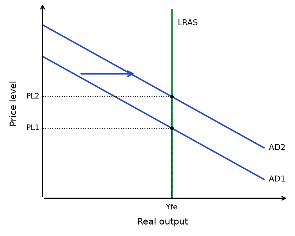
Read the diagram: Both AD curves intersect LRAS at Yfe. In this classical long-run model, higher AD raises the price level but does not raise potential output.
→ ↑ AD (long run, classical view) → PL rises from PL1 to PL2 → Y remains fixed at Yfe (full-employment output) → demand-side policy is powerless to raise output in the long run, only prices
On Keynesian LRAS (three sections)
Figure 2.20 Long-run aggregate supply
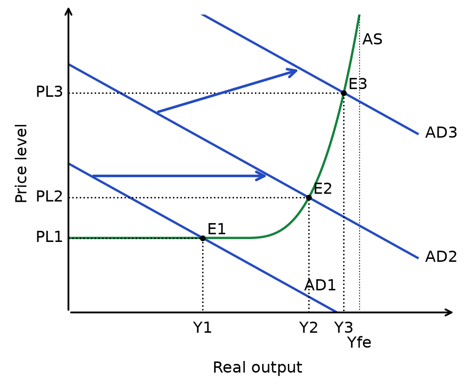
Read the diagram: Higher spending shifts AD right → find the new intersection on the single smooth AS curve → read real output and price level. With spare capacity, output responds strongly; near full employment, more adjustment occurs through prices. Yfe identifies capacity, not every short-run equilibrium.
| Section of Keynesian LRAS | Effect of ↑ AD |
|---|---|
| Horizontal (spare capacity) | ↑ Y, PL unchanged — not inflationary |
| Upward-sloping (approaching full employment) | Both ↑ Y and ↑ PL — some inflationary pressure |
| Vertical (full employment, Yfe) | ↑ PL only, Y unchanged — fully inflationary, identical to classical outcome |
Exam evaluation — the central AD/AS debate
→ Whether an increase in AD is desirable depends on how much spare capacity the economy has
In a recession (lots of spare capacity, e.g. on the Keynesian horizontal section) → expansionary demand-side policy raises output with minimal inflation risk → strong case for stimulus
Near or at full employment (vertical section on either view) → the same policy is purely inflationary → weak case for further demand-side stimulus; supply-side policy (shifting LRAS right) becomes the more appropriate tool for sustainable growth
Combining AD and AS shifts (higher-mark exam technique)
- Data response and essay questions often require analysing simultaneous changes in both AD and AS.
The rule
draw both shifts on the same diagram and identify the combined/net effect on PL and Y.
| Scenario | AD | AS | Net effect on PL | Net effect on Y |
|---|---|---|---|---|
| Both increase | ↑ | ↑ | Ambiguous (depends on relative size of shifts) | ↑ (unambiguous) |
| Both decrease | ↓ | ↓ | Ambiguous (depends on relative size of shifts) | ↓ (unambiguous) |
| AD ↑, AS ↓ | ↑ | ↓ | ↑ (unambiguous) | Ambiguous (depends on relative size of shifts) |
| AD ↓, AS ↑ | ↓ | ↑ | ↓ (unambiguous) | Ambiguous (depends on relative size of shifts) |
Exam tip
When both curves move in the same direction, the effect on real GDP (or PL, in the mixed cases) is certain, but the effect on the other variable is ambiguous and depends on the relative magnitude of the two shifts — a valuable point for evaluation ("the overall effect on the price level depends on whether the increase in AD outweighs the increase in AS").
In the standard diagram with upward-sloping SRAS and downward-sloping AD, simultaneous shifts often leave one outcome dependent on the relative shifts. State the curve assumptions; flat or vertical sections of AS can alter the result.
The starting position determines the balance between growth and inflation. Near capacity, further stimulus mainly raises prices; with simultaneous demand and supply shifts, assess their relative size before claiming a definite output outcome.
Rapid recap
AD–AS equilibrium determines real output and the price level. A positive demand shock raises output more with spare capacity; an adverse supply shock can lower output and raise prices together.
Diagram cue: locate both equilibria and explain the output and price-level effects.
Related chapters: Unit 2 chapter 2 (p. 32) · Unit 2 chapter 3 (p. 44)