Price elasticity of supply measures how easily output adjusts to a price change.
Must know
- PES equals percentage change in quantity supplied divided by percentage change in price.
- Spare capacity and stocks increase flexibility.
- Longer adjustment time often increases responsiveness.
Must know definitions
Price elasticity of supply (PES): measures the responsiveness of quantity supplied to a change in price.
Elastic supply: PES > 1; quantity supplied changes more than proportionately to a price change.
Inelastic supply: PES < 1; quantity supplied changes less than proportionately to a price change.
Unitary elastic supply: PES = 1; quantity supplied changes exactly proportionately to a price change.
Perfectly inelastic supply: PES = 0; quantity supplied does not change regardless of price.
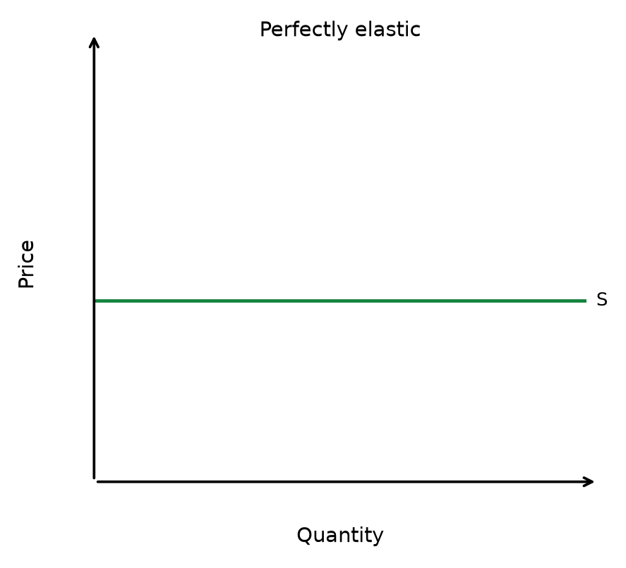
Perfectly elastic supply: PES = ∞; any quantity can be supplied at a given price.
Short run: time period where at least one factor of production is fixed.
Long run: time period where all factors of production are variable.
Spare capacity: unused resources that allow firms to increase output quickly.
Must know relationship: PES = %ΔQs / %ΔP.
Calculation: Qs is quantity supplied and P is price. PES has no unit: compare its value with 1 to judge responsiveness. Use percentage changes, not the ratio of the raw quantity and price changes.
Explain and apply
Mechanism in brief: A higher price encourages extra production. Existing stocks and spare capacity permit a quick response; long production cycles or specialised inputs restrict how far quantity can increase in the short run.
Distinguish: More elastic does not necessarily mean greater than one; PES can equal zero.
Use the extract: Identify spare capacity, stocks, production time and factor mobility; explain why these allow or prevent extra output.
The concept of price elasticity of supply
Price elasticity of supply (PES) measures the responsiveness of quantity supplied to a change in price.
- It shows how easily producers can adjust their output when the market price changes.
- A high PES means output can be scaled up or down quickly; a low PES means output is hard to change.
Calculation and interpretation of numerical values of PES
PES is calculated as the percentage change in quantity supplied divided by the percentage change in price: PES = %ΔQs / %ΔP.
- A value above 1 means supply is elastic; below 1 means inelastic; exactly 1 is unitary elastic.
- The extremes are perfectly elastic (PES = ∞) and perfectly inelastic (PES = 0).
PES is normally positive, because price and quantity supplied move in the *same* direction — a negative value would contradict the law of supply.
| PES value | Description | Meaning |
|---|---|---|
| ∞ | Perfectly elastic | A horizontal supply curve: supply is perfectly elastic at the given price. |
| > 1 | Elastic | A price change causes a more than proportionate change in quantity supplied |
| = 1 | Unitary elastic | A price change causes an exactly proportionate change in quantity supplied |
| 0 to 1 | Inelastic | A price change causes a less than proportionate change in quantity supplied |
| 0 | Perfectly inelastic | A price change causes no change in quantity supplied; supply is fixed |
PES is normally non-negative for the standard upward-sloping supply curve. A vertical supply curve has PES = 0; a horizontal supply curve is perfectly elastic.
Figure 1.16 PES comparison — Elastic at E
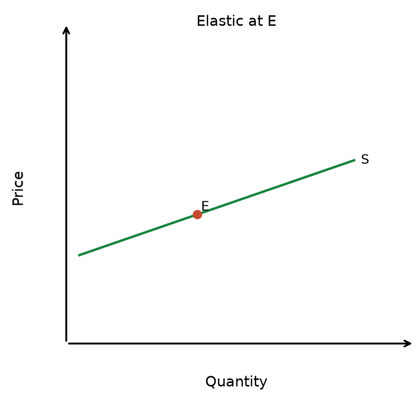
Interpretation: for this straight supply line, the positive price-axis intercept gives PES > 1 at E. The percentage quantity response exceeds the percentage price change.
Figure 1.17 PES comparison — Unit elastic at E
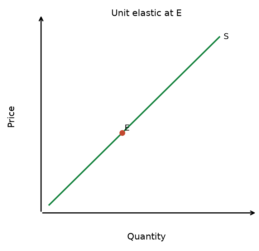
Interpretation: a straight supply line through the origin has PES = 1 at every positive point, regardless of its gradient.
Figure 1.18 PES comparison — Inelastic at E
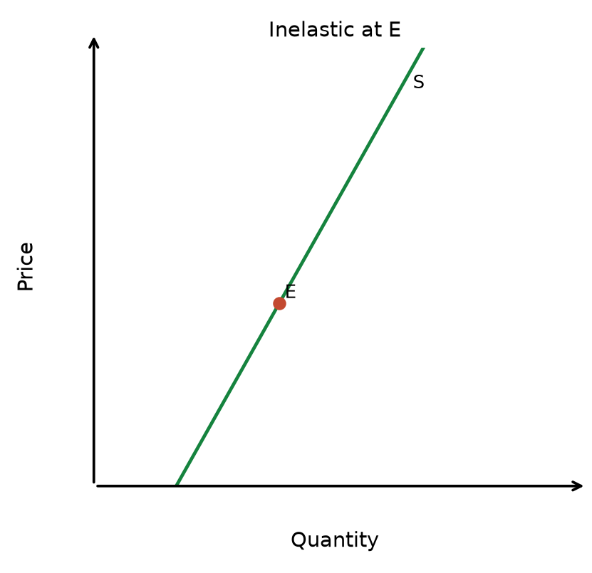
Interpretation: this straight supply line has a positive quantity-axis intercept, giving PES < 1 at E. The percentage quantity response is smaller than the percentage price change.
Read the diagram: The diagrams use the same reference point E and the same axis scales. For a linear curve at E, elasticity depends on both the slope and the price-to-quantity ratio. Do not compare elasticity from steepness alone across differently scaled diagrams.
Diagram link: PES comparison earlier in this topic. Apply the same labels and assumptions to the change described here.
Figure 1.19 PES comparison — Perfectly inelastic
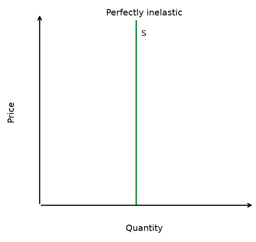
Figure 1.20 PES comparison — Perfectly elastic
Worked example: If the price of wheat rises by 15% and quantity supplied rises by 20%:
PES = %ΔQs / %ΔP = +20% / +15% = +1.33
Since PES is positive (price and quantity supplied moved in the same direction, as the law of supply predicts) and greater than 1, supply of wheat is relatively price elastic in this case.
PES is normally positive — a rising price raises quantity supplied, not lowers it. If your calculation gives a negative PES, you have most likely applied a demand-side movement (price up, quantity down) to supply by mistake.
Factors influencing PES
Whether supply is elastic or inelastic depends on how easily a firm can change its output — chiefly the time scale, spare capacity, and level of stocks.
- Firms with unused resources or storable stock can respond more quickly, tending to make supply more elastic.
- Perishable goods, full capacity, immobile resources and legal limits tend to make supply less elastic.
Barriers to entry matter too
low barriers let new firms enter and add to market supply.
| Factor | More elastic supply | Less elastic supply |
|---|---|---|
| Time scale | Long run — all factors of production can be adjusted | Short run — some factors are fixed |
| Spare capacity | Firm has unused resources (e.g. during a recession) | Operating at full capacity, no room to expand |
| Level of stocks | Goods are durable and can be stored (e.g. CDs) | Goods are perishable, hard to stock (e.g. apples) |
| Substitutability of factors | Labour and capital are mobile with transferable skills | Resources are scarce or immobile |
| Barriers to entry | Low barriers — new firms can enter easily | High barriers — difficult for new firms to enter |
| Legal constraints | No restrictions on increasing production | Legal limits prevent expansion of output |
The distinction between the short run and long run and its significance for PES
The short run is the time period where at least one factor of production is fixed, while in the long run all factors of production are variable.
- In the short run, supply is often less elastic because fixed factors, such as factory size, constrain expansion.
- In the long run, firms can build new factories, hire more workers, or adopt new technology, making supply more elastic.
the short run is defined by fixed factors, not by a set number of months — its length differs by industry.
| Short run | Long run | |
|---|---|---|
| Definition | Time period where some factors of production are fixed | Time period where all factors of production are variable |
| Ability to adjust output | Difficult — fixed factors limit production changes | Easy — all factors can be adjusted |
| PES | Usually less elastic than in the long run; PES need not be below 1 | Usually more elastic than in the short run; PES need not exceed 1 |
| Reason | Firms cannot quickly build new factories or hire more workers | Firms can expand capacity, enter new markets, or invest in technology |
Longer adjustment time can make supply more elastic, but physical or regulatory limits may persist. Judge the actual production constraint rather than assuming every industry's supply eventually becomes highly elastic.
Rapid recap
Mechanism: a higher price gives producers an incentive to expand, but stocks, spare capacity, factor mobility and production time determine the feasible quantity response.
Calculate and judge: PES = %ΔQs/%ΔP. More adjustment time often increases responsiveness; land, licences or specialised inputs may remain constraints.
Diagram cue: compare supply responsiveness using consistent axes and a stated point.
Related chapters: Unit 1 chapter 9 (p. 31) · Unit 1 chapter 16 (p. 80)