Elasticity measures responsiveness and helps predict revenue, demand and policy effects.
Must know
- PED compares percentage quantity and own-price changes.
- YED distinguishes normal and inferior goods.
- XED identifies substitutes and complements.
Must know definitions
Price elasticity of demand (PED): measures the responsiveness of quantity demanded to a change in price.
Income elasticity of demand (YED): measures the responsiveness of quantity demanded to a change in income.
Cross elasticity of demand (XED): measures the responsiveness of quantity demanded of one good to a change in the price of another good.
Total revenue (TR): price multiplied by quantity sold, TR = P × Q.
Inferior good: a good for which demand falls as income rises (YED < 0).
Normal good: a good for which demand rises as income rises (YED > 0).
Luxury good: a normal good where demand rises more than proportionately with income (YED > 1).
Must know relationship: PED = %ΔQd / %ΔP; YED = %ΔQd / %Δincome; XED = %ΔQd of A / %Δprice of B.
Calculation: Δ means change; Qd is quantity demanded and P is price. Use (new − original) / original × 100 for each percentage change unless another method is specified. Elasticity has no unit. Classify PED using its absolute size; retain the signs of YED and XED to identify the type of good or relationship.
Explain and apply
Mechanism in brief: With elastic demand, a price rise causes a proportionately larger quantity fall, reducing total revenue. With inelastic demand, quantity falls proportionately less, so total revenue rises; costs must also be considered for profit.
Distinguish: Use absolute PED for elastic versus inelastic; keep the signs of YED and XED.
Use the extract: Use the stated percentage changes, available substitutes and time period; connect the calculated sign and size to the decision.
The concepts of 'price', 'income' and 'cross-elasticities of demand'
Elasticity of demand measures how responsive quantity demanded is to a change in one of its determinants — price, income, or the price of another good.
- All three elasticities use the same logic (a ratio of percentage changes) but isolate a different cause.
- This lets economists predict how demand reacts to real-world changes such as a tax, a pay rise, or a rival's price cut.
- Elasticities matter because they turn the vague idea of "demand changes" into a precise, comparable number.
| Elasticity | Measures responsiveness of… | To a change in… |
|---|---|---|
| PED (price elasticity of demand) | Quantity demanded of a good | The price of that same good |
| YED (income elasticity of demand) | Quantity demanded of a good | Consumer income |
| XED (cross elasticity of demand) | Quantity demanded of good X | The price of a related good Y |
Formulae for PED, YED & XED
Each elasticity is calculated by dividing one percentage change by another, giving a single number whose size and sign reveal how strongly, and in what direction, demand responds.
if the price of bread rises 15% and quantity demanded falls 20%, PED = -20% ÷ 15% = -1.33.
Since the value ignoring the sign exceeds 1, bread is relatively price elastic in this case.
always divide the quantity change by the cause (price or income) — inverting the formula is a frequent lost mark.
| Elasticity | Formula |
|---|---|
| PED | % change in quantity demanded ÷ % change in price |
| YED | % change in quantity demanded ÷ % change in income |
| XED | % change in quantity demanded of good X ÷ % change in price of good Y |
Interpretation of numerical values of PED
PED is almost always negative, because price and quantity demanded move in opposite directions, so economists focus on its size ignoring the sign.
- A value greater than 1 (ignoring sign) means demand is elastic — very responsive to price.
- An absolute value below 1 means demand is inelastic: quantity demanded changes proportionately less than price.
A value of exactly 1 is unitary elastic
%ΔQd exactly matches %ΔP.
do not call a PED of -2 "smaller" than -0.5 — compare the absolute values.
| PED value | Type | Meaning |
|---|---|---|
| |PED| = ∞ | Perfectly elastic | Any price rise causes quantity demanded to fall to zero |
| PED < -1 | Price elastic | Quantity demanded changes proportionately more than price |
| PED = -1 | Unitary elastic | Quantity demanded changes by the same proportion as price |
| PED between 0 and -1 | Price inelastic | Quantity demanded changes proportionately less than price |
| PED = 0 | Perfectly inelastic | Quantity demanded does not change at all when price changes |
Figure 1.5 PED comparison — Elastic at E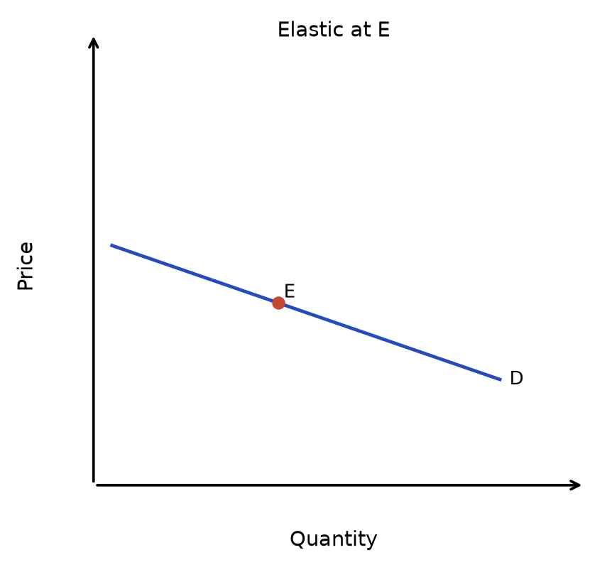 | Figure 1.6 PED comparison — Unit elastic at E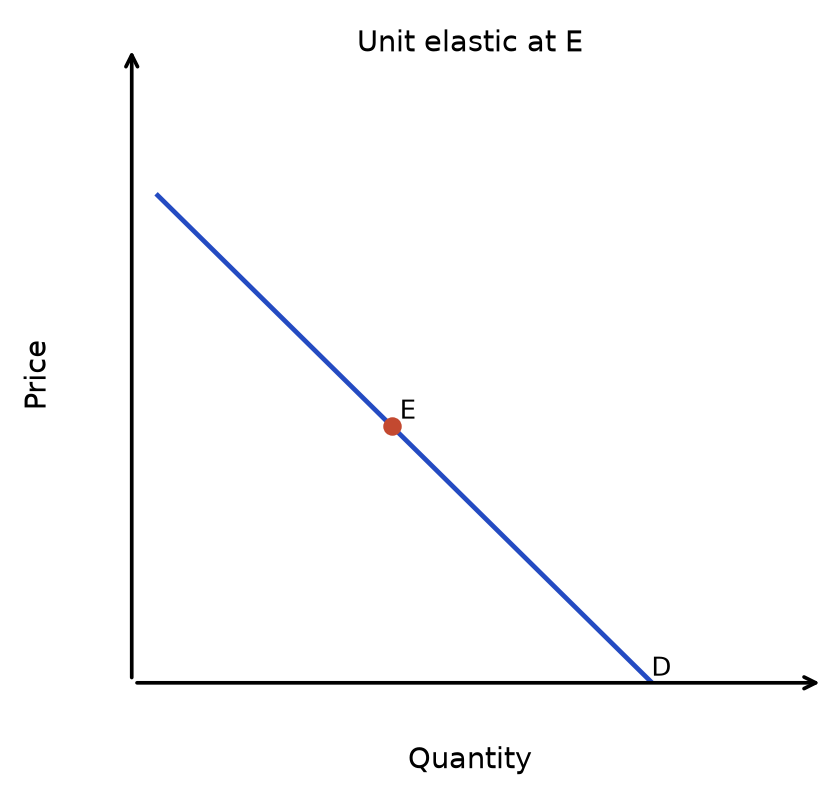 |
Figure 1.7 PED comparison — Inelastic at E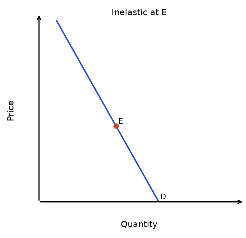 | Read the diagram: The diagrams use the same reference point E and the same axis scales. For a linear curve at E, elasticity depends on both the slope and the price-to-quantity ratio. Do not compare elasticity from steepness alone across differently scaled diagrams. The unit-elastic point on a straight line does not make the whole line unit elastic. A vertical curve has PED = 0; a horizontal curve is perfectly elastic at the indicated price. These are limiting cases. |
Figure 1.8 PED comparison — Perfectly inelastic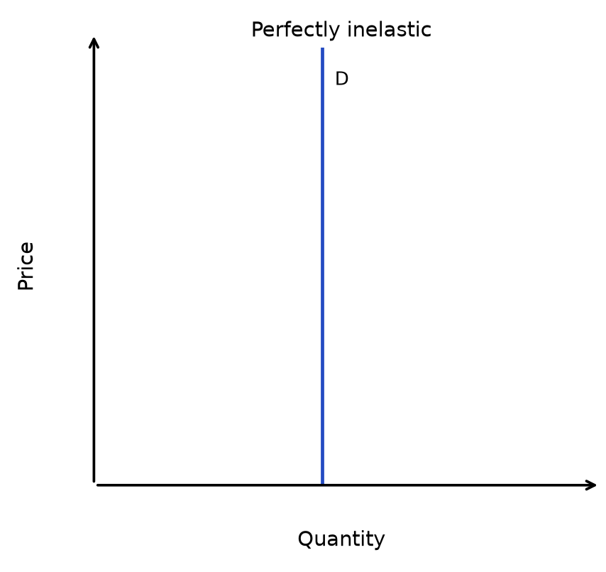 | Figure 1.9 PED comparison — Perfectly elastic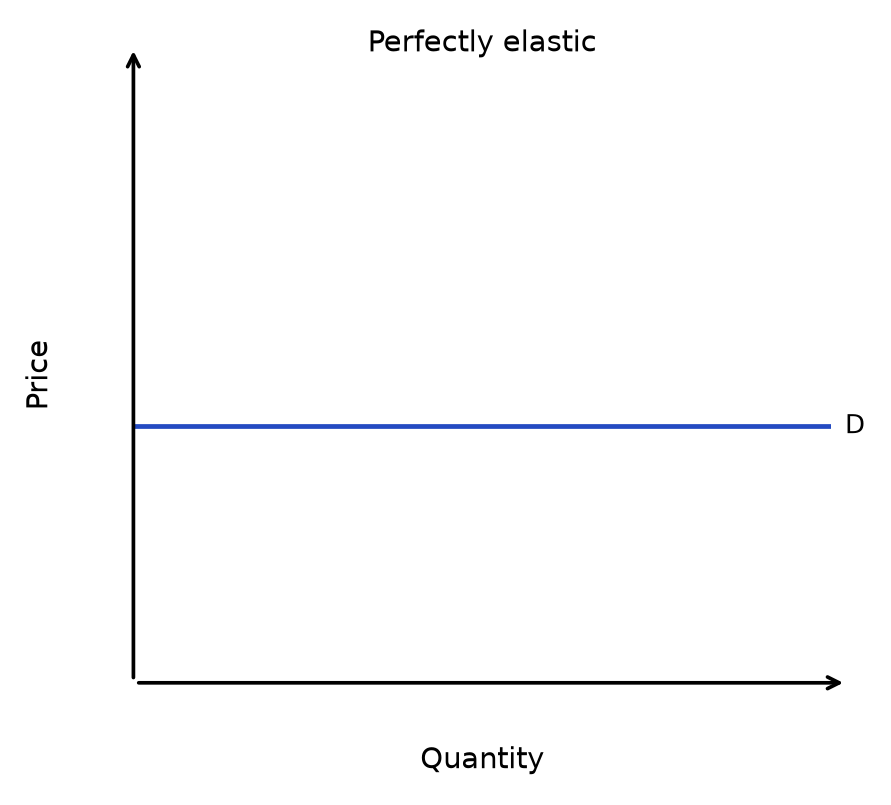 |
The factors influencing PED
Whether a good's demand is elastic or inelastic depends on structural features of the good and its market — above all the availability of substitutes and the proportion of income it takes up.
- These factors explain why identical percentage price rises produce very different responses across goods.
- A rise in the price of salt barely dents demand; the same percentage rise for a foreign holiday could sharply reduce it.
Time matters too
demand often becomes more price elastic over time as consumers find substitutes or change habits. Persistent constraints can still limit the response.
Brand loyalty can make demand less price elastic by reducing consumers’ willingness to switch. The effect is weaker when a close, trusted alternative is readily available, so a firm cannot assume that branding makes a price rise profitable.
| Factor | Explanation | Example |
|---|---|---|
| Substitutes | More and closer substitutes make it easier to switch away, so demand is more elastic; in the long run consumers have time to find substitutes, making demand more elastic than in the short run | Market for "white bread" (many substitutes) is more elastic than market for "bread" as a whole |
| Necessity | Necessities often have fewer substitutes and relatively low PED. Quantity still responds to price; affordability and the time period matter. | Electricity (inelastic) vs. holidays abroad (elastic) |
| Addictiveness/habit | Habit or addiction can make quantity demanded respond relatively little to price, especially in the short run; this does not imply PED = 0. | Cigarettes |
| Proportion of income | Other things equal, a larger budget share tends to make demand more price sensitive because a price rise has a greater effect on purchasing power. This does not alone establish whether absolute PED exceeds 1. | A car purchase usually takes a larger budget share than a magazine; substitution options and necessity also matter. |
| Durability | Long-lasting goods can be delayed or repaired instead of replaced, making demand more elastic | Washing machine |
| Time of use (peak/off-peak) | Peak-time users may have fewer alternatives, making demand relatively less elastic. The response still depends on journey purpose, available substitutes and adjustment time. | A commuter with fixed working hours may be less responsive than a leisure traveller able to change departure time. |
How to calculate total revenue
Total revenue (TR) is the total income a firm receives from selling its output: TR = P × Q.
- For a movement along an unchanged demand curve, the effect of a small price change on revenue depends on PED at the relevant point. For a sizeable change, calculate before-and-after P × Q or use elasticity measured over that range.
- A firm cannot judge the impact of a price change on its income without first knowing the relevant PED.
How PED varies along a straight-line demand curve
PED is not constant along a straight-line demand curve — it changes continuously as price and quantity move along the line, even though the slope (gradient) stays the same.
- Demand is elastic in the top half (high price, low quantity): a given absolute price change is a small percentage of the initial price, while its associated quantity change is a large percentage of the initial quantity.
- Demand is inelastic in the bottom half (low price, high quantity).
- At the exact midpoint, PED = -1 (unitary elastic).
constant slope does not mean constant elasticity — slope and elasticity are different things.
Figure 1.10 PED along a straight demand curve
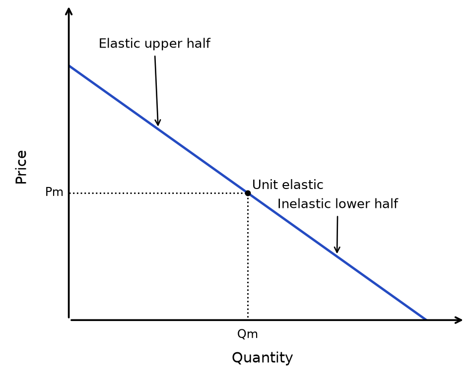
Read the diagram: The slope is constant but PED varies because the price-to-quantity ratio changes. The midpoint is unit elastic; higher-price points are elastic and lower-price points are inelastic.
The relationship between PED and total revenue
Because TR = P × Q, the revenue effect depends on PED over the relevant price range. Constant unit-elastic demand gives unchanged TR. A straight demand curve is unit elastic only at its midpoint, where TR peaks; moving away from that point reduces TR.
- Useful application: use PED to explain how a price change affects total revenue, holding other demand determinants constant.
- Firms use it directly to decide whether to raise or cut prices.
- Within an inelastic range, a price rise increases TR; within an elastic range, a price cut increases TR. A large change may cross into another elasticity range.
| PED | Price rises | Price falls |
|---|---|---|
| Inelastic (< 1) | TR rises | TR falls |
| Unitary throughout the relevant price range (= 1) | TR unchanged | TR unchanged |
| Elastic (> 1) | TR falls | TR rises |
Figure 1.11 Revenue relationships — panel 1
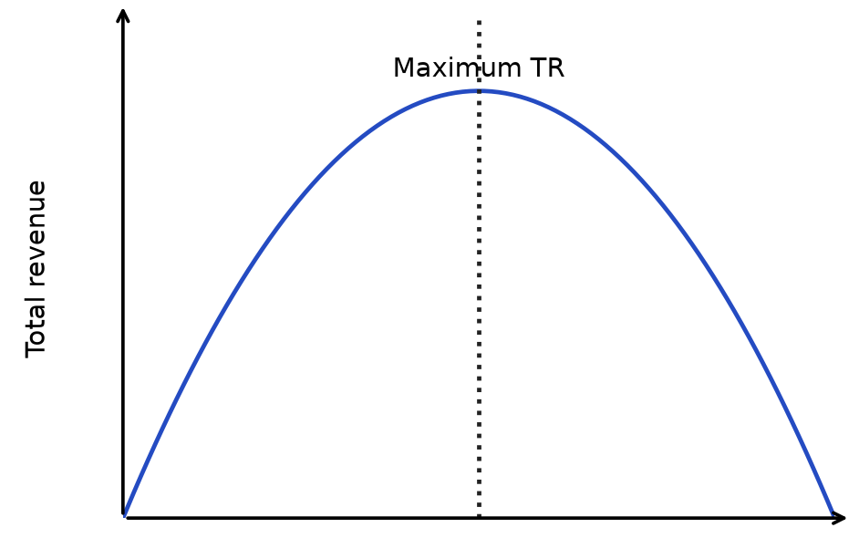
Figure 1.12 Revenue relationships — panel 2
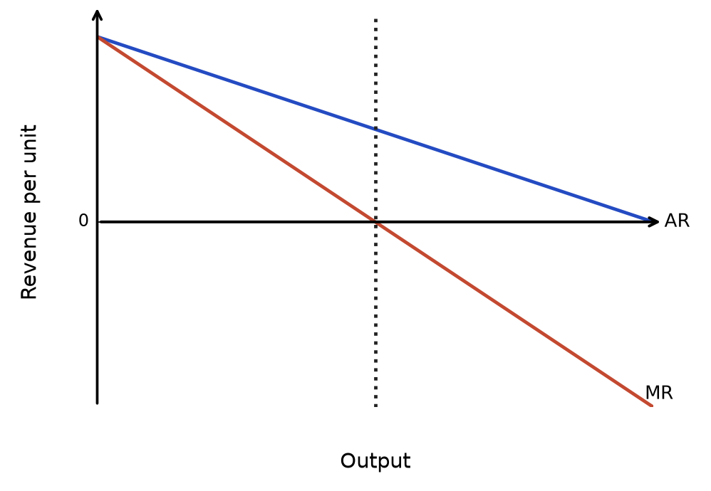
Read the diagram: Unit 1 focus — TR reaches its maximum at the unit-elastic point on straight-line demand. Bridge to Unit 3 — MR is extra revenue from one more unit: TR rises when MR > 0, falls when MR < 0, and is maximised where MR = 0.
Interpretation of numerical values of YED
Income elasticity of demand (YED) shows how demand responds to a change in consumer income, and its sign matters as much as its size.
- A negative YED signals an inferior good — demand falls as income rises, e.g. supermarket value-brand ranges as shoppers switch to branded goods when they can afford to.
- A positive YED signals a normal good; a YED above +1 signals a luxury good.
- During periods of economic growth, firms often shift production towards income-elastic luxury goods and away from inferior goods.
| YED value | Type | Example |
|---|---|---|
| YED < 0 | Inferior good — demand falls as income rises | Value-brand supermarket goods |
| YED = 0 | Perfectly income inelastic | No income response in the stated range |
| YED between 0 and +1 | Normal good, income inelastic | Bread, basic clothing |
| YED = +1 | Normal good, unit income elastic | Demand rises proportionately with income |
| YED > 1 | Normal good, income elastic (luxury good) | Foreign holidays |
Perfectly income-elastic demand
Perfectly income-elastic demand is the limiting case in which quantity demanded is infinitely responsive to income at a particular income level, with the good’s price and other influences held constant. The magnitude of YED tends to infinity; this is different from an ordinary income-elastic good, whose YED is finite and greater than 1.
For a normal good, an arbitrarily small percentage increase in income can be associated with a finite increase in quantity demanded in this limiting model. It is a theoretical benchmark, not a claim that a familiar good normally behaves this way.
YED = % change in quantity demanded ÷ % change in income. For illustration, 10% ÷ 0.1% = 100; 10% ÷ 0.01% = 1,000. As the denominator approaches zero while the numerator remains non-zero, the ratio becomes arbitrarily large.
These ratios illustrate the limit, not observed demand data. Do not divide by an income change of exactly zero and call the result a finite measured elasticity: that calculation is undefined.
Distinguish: perfectly income-inelastic demand has YED = 0, so quantity demanded does not respond to an income change. Perfectly income-elastic demand describes the opposite limiting response.
Interpretation of numerical values of XED
Cross elasticity of demand (XED) shows how demand for good X responds to a price change in a different good Y, and again the sign reveals the relationship between the two goods.
- Negative XED = complements: a rise in the price of one good reduces demand for the other, other things equal.
- Positive XED = substitutes — goods that replace one another, so a price rise in one increases demand for the other.
Strength also varies
For a given percentage change in the other good’s price, a larger absolute XED means a larger percentage change in demand. Positive XED indicates substitutes; negative XED indicates complements.
| XED value | Type | Example |
|---|---|---|
| XED < 0 | Complements — demand for X falls if price of Y rises | Strawberries and cream |
| XED = 0 | Unrelated goods | Bus fares and tables |
| XED > 0 | Substitutes — demand for X rises if price of Y rises | Two rival cola brands |
| Strength | Complements | Substitutes |
|---|---|---|
| Close | For a given % fall in Y’s price, a larger % rise in demand for X (magnitude of XED). | For a given % rise in Y’s price, a larger % rise in demand for X (magnitude of XED). |
| Weak | For a given % fall in Y’s price, a smaller % rise in demand for X (magnitude of XED). | For a given % rise in Y’s price, a smaller % rise in demand for X (magnitude of XED). |
The significance of PED, YED & XED for firms, consumers and the government
Firms, consumers and the government all use elasticity values differently.
- Firms rely on PED to set prices for maximum revenue and on XED to anticipate rivals' pricing moves.
- The government uses PED to predict how the burden of a tax, or the benefit of a subsidy, is shared between firms and consumers.
YED matters for firms' long-term planning
a business selling income-elastic luxury goods is far more exposed to a downturn than one selling income-inelastic necessities.
| Elasticity | User | Significance |
|---|---|---|
| PED | Firms | Guides pricing strategy: if demand is inelastic, raising price increases TR; if elastic, raising price reduces TR |
| PED | Government | Tax and subsidy incidence depends on the relative price elasticities of demand and supply. The less elastic side of the market generally bears more of a tax and receives more of a subsidy. |
| YED | Firms | Warns of exposure to the economic cycle: income-elastic (luxury) goods see demand fall sharply in a recession, while income-inelastic goods are more stable |
| XED | Firms | Reveals how many close competitors a firm faces and how its sales will be affected by a competitor's price change |
An elasticity estimate applies to a particular market, price range and time period. Substitution and adjustment usually become easier over time, so a short-run estimate may overstate the lasting revenue gain from a price rise.
Rapid recap
Calculate: PED = %ΔQd/%ΔP; YED = %ΔQd/%Δincome; XED = %ΔQd(A)/%ΔP(B). Use the same period and state what each percentage measures.
Interpret: use absolute PED for responsiveness; retain YED and XED signs to classify the good or relationship. Along a standard straight demand curve, PED changes with position.
Apply: a small price rise raises TR when demand is inelastic and lowers TR when elastic, holding demand fixed. Revenue is not profit; costs and the relevant price range also matter.
Diagram cue: link the relevant PED range to the price change and total revenue.
Related chapters: Unit 1 chapter 11 (p. 46) · Unit 1 chapter 16 (p. 80)
Why this connects: Use PED to explain revenue effects, then combine PED with PES to explain tax incidence. Responsiveness determines both how much quantity changes and who bears the price wedge.