Aggregate supply distinguishes current production costs from long-run productive capacity.
Must know
- SRAS responds to unit costs.
- LRAS reflects productive potential.
- Classical and Keynesian models differ in their adjustment assumptions.
Must know definitions
Aggregate supply (AS) — the total amount of goods and services (real output) produced and supplied by an economy's firms at a particular price level over a period of time.
Short-run aggregate supply (SRAS) — the relationship between the price level and real output supplied while nominal wages and some input prices have not fully adjusted; usually upward-sloping.
Long-run aggregate supply (LRAS) — the relationship between the price level and real output after wages and input prices have adjusted; its shape depends on the model’s assumptions.
Classical LRAS — a vertical curve at sustainable potential output (Yfe). Flexible wages and prices restore this output in the model’s long-run equilibrium.
Keynesian LRAS — an LRAS curve with a horizontal section (spare capacity), an upward-sloping section, and a vertical section (full employment), reflecting the view that the economy can remain below full-employment output for extended periods.
Spare capacity — underused labour or capital that can allow output to rise with limited extra inflationary pressure.
Full-employment output (Yfe) — sustainable potential output with resources used at normal capacity. Frictional and structural unemployment can remain; actual output may temporarily exceed this level.
Productivity — output per worker per hour worked.
"Red tape" — a colloquial term for excessive government regulation that raises firms' costs of compliance and can reduce AS.
Explain and apply
Mechanism in brief: Higher energy costs increase firms' costs at each output, shifting SRAS left. Better skills can increase potential production and shift LRAS right, but only after training is completed and skills are used productively.
Distinguish: A shift in LRAS does not mechanically guarantee an immediate shift in SRAS; Keynesian AS has different sections.
Use the extract: Distinguish a change in current production costs from a change in productive capacity; identify the resource or technology affected.
Definition reminder: Aggregate supply (AS)
The AS curve
SRAS is upward-sloping in the short-run AD–AS model. The Keynesian AS model below is a separate, continuous curve with a flat region, a rising region and a near-vertical full-employment region.
- With upward-sloping SRAS, a higher price level encourages more real output at given input costs. The response on Keynesian AS varies with spare capacity.
Figure 2.9 Movement along SRAS
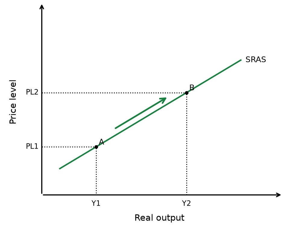
Read the diagram: The price level changes, holding other influences fixed. The arrow shows movement from A to B along the same SRAS curve. Real output is labelled Y and the price level PL; this is not a shift of the curve.
Why SRAS slopes upward: at a higher price level, firms can earn higher profits (assuming costs are relatively fixed in the short run) → firms are willing and able to supply more output → upward-sloping SRAS.
Movement along vs shift of AS
| Change | Cause | Effect on diagram |
|---|---|---|
| Movement along AS | A shift in the AD curve causes a new equilibrium price level, which firms respond to by adjusting output along the existing AS curve | Expansion (↑ output as PL rises) or contraction (↓ output as PL falls) along the same curve |
| Shift of AS | A change in the conditions of supply at every price level (not caused by AD) | Entire curve shifts right (↑ AS) or left (↓ AS) |
→ Change in AD → new equilibrium PL → movement along the AS curve (NOT a shift)
→ Change in firms' costs of production or supply conditions → shift of the entire AS curve
Figure 2.10 Shifts of SRAS — Increase
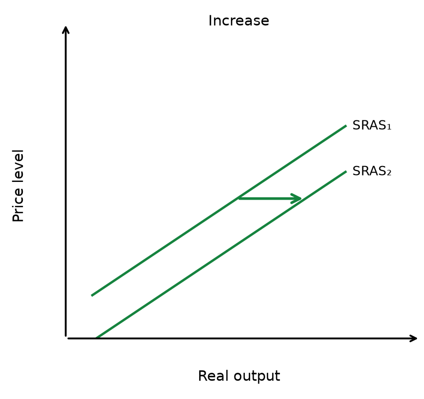
Figure 2.11 Shifts of SRAS — Decrease
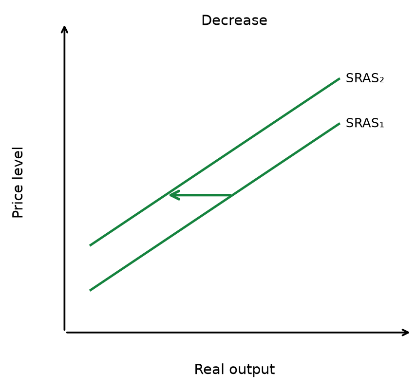
Read the diagram: Each panel shows a change in a non-price determinant, holding other influences fixed. The arrow runs from curve 1 to curve 2: an increase is a rightward shift; a decrease is a leftward shift. Compare quantities at the same vertical-axis value.
Common mistake: a very common mistake is treating a change in AD as if it shifts the AS curve.
Remember
AD changes cause movement along AS (a new equilibrium point); only changes in the conditions of supply (costs, technology, regulation) cause AS itself to shift.
Short-run aggregate supply (SRAS)
Factors influencing SRAS
- SRAS shifts when firms' costs of production change at every price level.
Cost of employment (wages)
Mechanism: ↑ wages → ↑ firms' costs of production → firms supply less at each PL → SRAS shifts left
Arrow chain: ↑ wages → ↑ costs → ↓ SRAS (shift left)
Labour productivity
Mechanism: ↑ productivity → same output for lower unit labour cost → ↓ costs per unit → SRAS shifts right
Arrow chain: ↑ labour productivity → ↓ unit costs → ↑ SRAS (shift right)
Commodity / raw material prices
Mechanism: ↑ price of oil or key raw materials → ↑ input costs → SRAS shifts left
Arrow chain: ↑ commodity prices → ↑ costs of production → ↓ SRAS (shift left)
Exchange rate (for imported inputs)
Mechanism: ↓ exchange rate (depreciation) → imported raw materials become more expensive → ↑ costs → SRAS shifts left
Arrow chain: ↓ exchange rate → ↑ cost of imported inputs → ↓ SRAS (shift left)
Indirect taxes
Mechanism: ↑ indirect tax (e.g. VAT, excise duty) → ↑ effective cost of supplying goods → SRAS shifts left
Arrow chain: ↑ indirect tax → ↑ costs → ↓ SRAS (shift left)
Subsidies
Mechanism: ↑ government subsidies to firms → ↓ effective cost of production → SRAS shifts right
Arrow chain: ↑ subsidies → ↓ costs → ↑ SRAS (shift right)
Government regulation ("red tape")
Mechanism: ↑ regulation (environmental laws, business compliance costs) → ↑ costs of compliance → SRAS shifts left; deregulation → ↓ costs → SRAS shifts right
Arrow chain: ↑ regulation → ↑ compliance costs → ↓ SRAS (shift left)
Exam tip: Notice that SRAS shifters are almost entirely cost-side factors.
- Rising input prices may shift SRAS left, but a shock can affect demand as well as supply. A weaker currency can raise imported-input costs and also influence net exports; business-tax changes may affect investment. Identify each channel supported by the extract.
Long-run aggregate supply (LRAS)
- There are two competing views of the shape of the LRAS curve — classical and Keynesian. The spec requires you to understand both, and to know when each is more appropriate to use.
Classical LRAS
Classical economists believe the LRAS curve is perfectly (vertical) inelastic.
- They argue that in the long run, all markets clear (wages and prices are flexible), meaning there can be no output gap in the long run — the economy always returns to producing at its maximum potential level of output.
Figure 2.12 Long-run aggregate supply
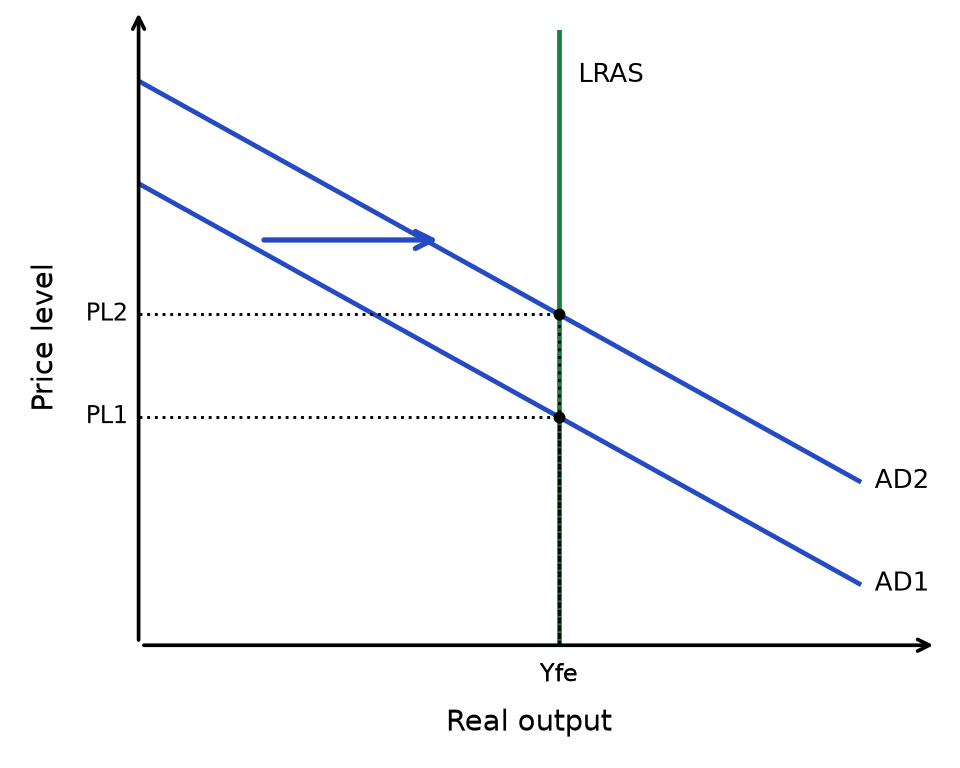
Read the diagram: Both AD curves intersect LRAS at Yfe. In this classical long-run model, higher AD raises the price level but does not raise potential output.
Key implication: because LRAS is vertical, a shift in AD only changes the price level in the long run — it has no effect on real output.
This is a critical exam point
classical economists believe demand-side policy (e.g. fiscal stimulus) cannot increase output in the long run, only prices.
→ Classical view: ↑ AD (long run) → ↑ PL only → no change in real GDP (output is fixed at Yfe)
Keynesian LRAS
Keynesian economists believe it is possible to have long-run equilibrium where markets do not clear, so there can be spare capacity in the economy even in the long run.
- The Keynesian LRAS curve has three distinct sections.
Figure 2.13 Long-run aggregate supply
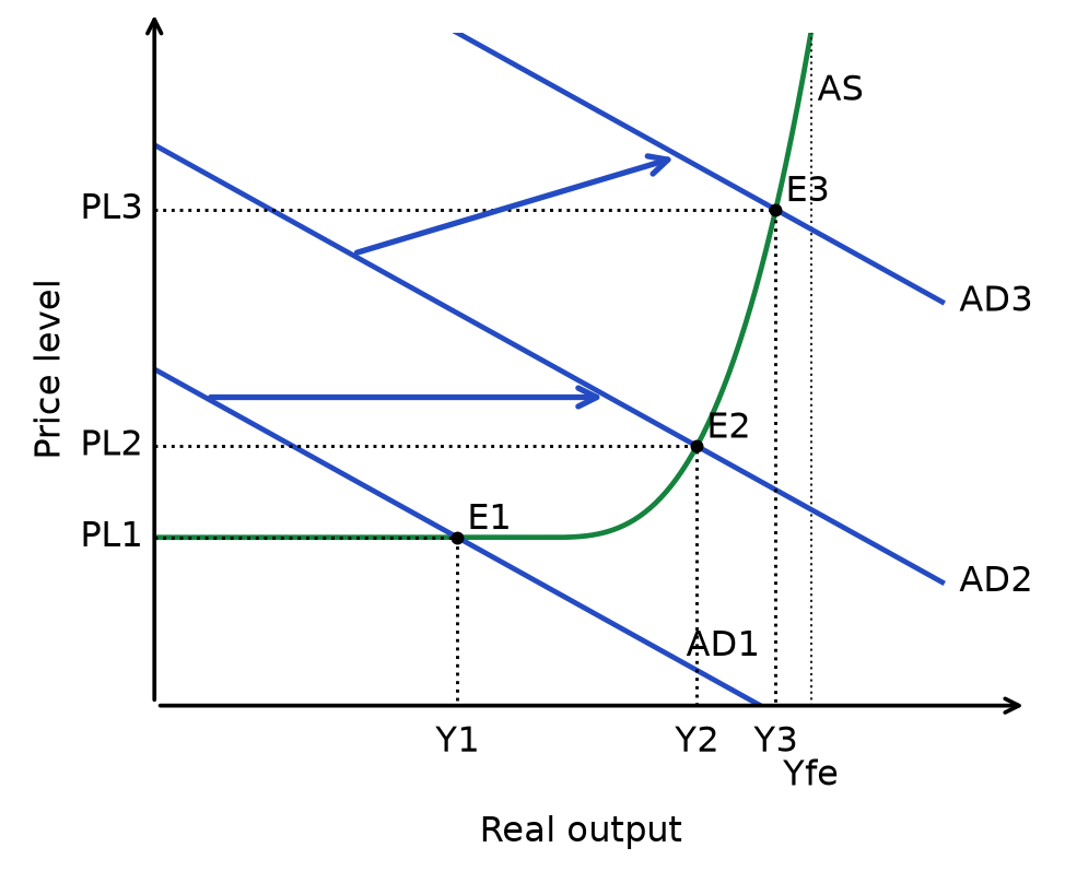
Read the diagram: Higher spending shifts AD right → find the new intersection on the single smooth AS curve → read real output and price level. With spare capacity, output responds strongly; near full employment, more adjustment occurs through prices. Yfe identifies capacity, not every short-run equilibrium.
| Section | Economic condition | Effect of ↑ AD |
|---|---|---|
| Horizontal (flat) | Lots of spare capacity; high unemployment of resources | ↑ AD → ↑ real output with no change in price level (not inflationary) |
| Upward-sloping (intermediate) | Spare capacity being used up; some bottlenecks emerging | ↑ AD → ↑ real output AND ↑ price level (some inflationary pressure) |
| Vertical | Full employment; all factors of production fully utilised | ↑ AD → ↑ price level only, no change in real output (fully inflationary) — identical to the classical case |
Exam tip — this is a high-value evaluation point: the Keynesian LRAS shows that the effect of an AD-side policy (e.g. expansionary fiscal or monetary policy) on inflation vs growth depends entirely on how much spare capacity the economy has.
- An economy in a deep recession (lots of spare capacity) can expand AD with little inflation risk; an economy near full employment will see mostly price rises from the same policy.
Classical vs Keynesian LRAS comparison
| Classical LRAS | Keynesian LRAS | |
|---|---|---|
| Shape | Vertical at potential output (Yfe) | Horizontal, then upward-sloping, then vertical |
| Assumption | Wages and prices are fully flexible; markets always clear | Wages and prices can be "sticky"; markets may not clear, especially downward |
| Long-run output gap | Never possible — economy always returns to Yfe | Possible — economy can remain below Yfe indefinitely (e.g. a prolonged recession) |
| Policy implication | In this vertical-LRAS model, a pure AD increase does not raise long-run capacity. Policies that also improve investment, skills or infrastructure may shift LRAS. | Demand-side policy CAN raise output long-run if there is spare capacity |
Common mistake: don't apply the classical "demand-side policy can't raise long-run output" conclusion to a Keynesian LRAS with spare capacity — the two models give opposite policy implications, so state which view you are using.
Factors influencing LRAS
- LRAS shifts when the quantity or quality of the factors of production changes — this is equivalent to shifting the economy's PPF outward.
Technology
Mechanism: ↑ investment in technology → firms produce more output from the same inputs, or improve quality → ↑ LRAS
Arrow chain: ↑ technology → ↑ productive capacity → ↑ LRAS (shift right)
Productivity
Mechanism: ↑ output per worker per hour worked → same labour force produces more → ↑ LRAS
Arrow chain: ↑ productivity → ↑ potential output → ↑ LRAS (shift right)
Quantity/quality of factors of production
Mechanism: ↑ capital stock, ↑ number of workers, or ↑ quality of resources (e.g. more fertile land, better machinery) → ↑ LRAS
Arrow chain: ↑ quantity/quality of factors → ↑ LRAS (shift right)
Education and skills
Mechanism: ↑ investment in education and training → ↑ quality of human capital → workers more productive and versatile → ↑ LRAS (long time lag)
Arrow chain: ↑ education/skills → ↑ quality of labour → ↑ LRAS (shift right)
Government regulation
Mechanism: ↓ excessive regulation ("red tape") → ↓ compliance burden on firms → firms can be more efficient → ↑ LRAS; ↑ regulation → ↓ LRAS
Arrow chain: ↓ regulation → ↑ efficiency → ↑ LRAS (shift right)
Competition policy
Mechanism: ↑ effective competition policy → firms forced to be more efficient/productive to avoid being competed out of business → ↑ LRAS
Arrow chain: ↑ competition → ↑ efficiency → ↑ LRAS (shift right)
Demography and net migration
Mechanism: ↑ net inward migration (especially of working-age people) → ↑ size of labour force → ↑ LRAS
Arrow chain: ↑ net migration (working-age) → ↑ labour force → ↑ LRAS (shift right)
Exam tip: LRAS shifters are almost always supply-side policy territory (education, infrastructure, deregulation, competition policy, migration policy).
- If a question asks about "long-run growth" or "increasing potential output," it is asking about LRAS shifters, not AD components.
SRAS vs LRAS comparison
| SRAS | LRAS | |
|---|---|---|
| Time frame | Short run — wages and some input prices have not fully adjusted | Long run — wages and input prices can fully adjust |
| Slope | Usually upward-sloping in the short-run AD–AS model | Classical: vertical. Keynesian: horizontal-then-upward-then-vertical |
| Shifters | Cost-side factors: wages, commodity prices, exchange rate, indirect taxes, subsidies, regulation | Factors affecting quantity/quality of resources: technology, productivity, education, migration, competition policy |
| Relationship to AD | AD shifts cause movement ALONG SRAS | AD shifts do NOT change output once on the vertical section of LRAS (classical or Keynesian full-employment) |
Relationships between LRAS and SRAS shifts
- A productivity improvement may shift both LRAS and SRAS right: it raises potential output and lowers unit costs. However, do not assume every change in long-run capacity produces an immediate short-run cost change. State the mechanism and timing. A temporary input-price change can shift SRAS without changing LRAS.
A change in productive capacity can affect current costs as well, but its effect on SRAS depends on when new resources become usable and on what happens to input prices and productivity.
Example
↑ productivity (an LRAS shifter) → workers produce more output per hour → ↓ unit labour cost → firms' short-run costs also fall → SRAS shifts right too
Example
↑ investment in technology → potentially ↑ productive capacity as the technology becomes usable → if it also lowers unit costs, SRAS shifts right. The timing and scale of the two effects may differ.
→ SRAS shift ≠ LRAS shift (not necessarily true): a change in short-run production costs does not change the economy's underlying productive capacity
Example
↓ oil price (a SRAS shifter) → ↓ firms' short-run costs → SRAS shifts right → but the economy's quantity/quality of factors of production (labour, capital, technology) is unchanged → LRAS does NOT shift
Example
Currency appreciation causing cheaper imported inputs → SRAS shifts right → but this is a temporary cost change, not a change in the economy's productive potential → LRAS unaffected
| Type of shifter | Shifts SRAS? | Shifts LRAS? | Reasoning |
|---|---|---|---|
| ↑ Productivity | Yes | Yes | Lower unit costs (SRAS) AND higher potential output (LRAS) |
| ↑ Technology/investment | May do, as unit costs fall | Yes | Can expand capacity as investment becomes usable; SRAS shifts right if unit costs fall. |
| ↑ Education and skills | Yes (eventually) | Yes | Improves both current efficiency and long-run capacity |
| ↓ Oil/commodity prices | Yes | No | Only affects current costs, not productive capacity |
| Currency appreciation (cheaper imports) | Yes | No | Temporary cost effect, not a capacity change |
| ↓ Indirect tax / ↑ subsidy | Yes | No | Changes the cost firms face, not what they are capable of producing |
| ↑ Wages | Yes | No | A cost shock, not a productivity or capacity change |
Common mistake: don't assume every SRAS shifter also shifts LRAS. A temporary input-cost change can shift SRAS without changing productive capacity. A change in the quantity or quality of factors of production can shift LRAS and may also shift SRAS, depending on its effect on unit costs and when the resources become usable.
Exam tip — this is a strong evaluation point: when asked to assess a policy's impact on AS, always check whether it changes underlying productive capacity (technology, quality/quantity of factors) as well as costs.
A policy that only lowers costs (e.g. a fuel subsidy) gives a temporary SRAS boost but does NOT raise the economy's long-run potential output — whereas a policy that raises productivity or invests in capital/education raises both, giving a more sustainable increase in AS.
Exam explanation stems: aggregate supply
Use these ready-made stems to explain AS in exam answers:
SRAS shift via costs
↑ price of oil (a key commodity) → ↑ firms' costs of production → firms supply less output at each price level → SRAS shifts left → ↓ real GDP and ↑ price level (stagflation risk).
SRAS shift via exchange rate
Depreciation → imported raw materials become dearer in domestic currency → firms’ production costs rise → SRAS shifts left, raising the price level and reducing real output, other things equal.
Classical LRAS — a vertical curve at sustainable potential output (Yfe). Flexible wages and prices restore this output in the model’s long-run equilibrium.
Because classical economists view LRAS as vertical, an increase in AD (e.g. from expansionary fiscal policy) can only raise the price level in the long run — it cannot raise real output beyond Yfe. Use this to evaluate demand-side policy as a long-run growth tool.
Keynesian LRAS — spare capacity argument
If the economy has significant spare capacity (operating on the horizontal section of Keynesian LRAS), an increase in AD can raise real output with little to no increase in the price level. This justifies demand-side stimulus during a recession without much inflation risk. As the economy approaches full employment, the same AD increase becomes increasingly inflationary.
LRAS shift via supply-side policy
↑ government spending on education and training → ↑ quality of human capital (long time lag) → ↑ productivity → ↑ LRAS → economy can sustain higher real GDP at every price level without additional inflationary pressure — a more sustainable route to long-run growth than demand-side stimulus alone.
LRAS vs SRAS shift — distinguishing genuine capacity growth from a temporary cost shock: ↑ productivity raises LRAS (more potential output) AND lowers unit costs, so SRAS shifts right too — a durable improvement in AS. By contrast, a fall in oil prices only shifts SRAS right (lower costs), leaving LRAS unchanged, because the economy's underlying productive capacity has not increased. Use this distinction to evaluate whether a policy or shock produces a temporary or a permanent improvement in AS.
Distinguish a temporary cost shock from a lasting capacity change. Supply-side improvements may take years and require complementary investment; a policy announcement does not itself increase productive potential.
Rapid recap
SRAS shifts with current production costs; LRAS shifts with resources, technology and productive capacity. A price-level change alone causes movement along the relevant supply curve.
Diagram cue: distinguish an SRAS cost shift from an LRAS capacity shift.
Related chapters: Unit 2 chapter 4 (p. 55) · Unit 2 chapter 9 (p. 90)