Economic performance requires several indicators because no single measure captures output, stability and living standards.
Must know
- Use real and per-capita measures appropriately.
- Distinguish inflation deflation and disinflation.
- Separate unemployment underemployment and current-account balances.
Quantitative methods reference — p. 98
Find a measure: Economic Growth | Inflation | Employment and Unemployment | Balance of Payments
Growth and living standards — p. 6
Inflation — p. 10
Employment and unemployment — p. 16
Balance of payments — p. 25
Must know definitions
Economic growth — an increase in the real value of goods and services produced by an economy over time.
Real GDP — the total value of all final goods and services produced within a country's borders, adjusted for inflation.
Nominal GDP — GDP measured at current market prices, not adjusted for inflation.
GDP per capita — total GDP divided by the population of a country.
GNI (Gross National Income) — GDP plus primary income received by residents from abroad minus primary income paid to non-residents. Primary income includes relevant earnings from employment and investment; citizenship is not the criterion.
PPP (Purchasing Power Parity) — an adjustment to GDP/GNI that accounts for differences in the cost of living between countries.
Technical recession — two consecutive quarters of negative economic growth.
Inflation — a sustained increase in the general price level over time.
Deflation — a sustained decrease in the general price level.
Disinflation — a fall in the rate at which the general price level is rising.
CPI (Consumer Price Index) — a measure of the average change in prices of a representative basket of goods and services purchased by households.
RPI (Retail Price Index) — an alternative measure of inflation that includes mortgage interest payments and council tax.
PPI (Producer Price Index) — a measure of the average change in prices charged by domestic producers for their output; a leading indicator of future consumer inflation.
Unemployment — people without work who sought work in the previous four weeks and can start within two weeks; also those without work who have a job arranged to start within two weeks.
Underemployment — people who have a job but whose labour is not fully utilised (e.g. part-time workers seeking full-time work).
Economically inactive — people outside employment who do not meet the unemployment criteria because they are not actively seeking work and/or are unavailable to start. State the age band used in the data.
Balance of payments — a record of economic transactions between residents and non-residents over a stated period.
Current account — records trade in goods and services, primary income (including investment income) and secondary income (current transfers).
Current account deficit — total current-account payments exceed receipts across trade in goods and services, primary income and secondary income. A trade deficit is only one possible component.
Current account surplus — total current-account receipts exceed payments across trade in goods and services, primary income and secondary income.
Net migration — the difference between immigrants entering and emigrants leaving a country.
Must know relationship: Annual inflation = (CPI this year − CPI last year) / CPI last year × 100.
Calculation: CPI is an index, not a percentage inflation rate. Compare the same month or quarter one year apart for annual inflation. A fall from 6% to 4% is a fall of 2 percentage points; prices are still rising.
Explain and apply
Mechanism in brief: Nominal output combines price and volume changes. Deflating it isolates estimated real output; dividing by population gives an average. Neither calculation shows how income is distributed or captures every aspect of wellbeing.
Distinguish: A current-account deficit is broader than a trade deficit; a falling unemployment rate need not mean more people are employed.
Use the extract: Check real versus nominal values, totals versus per-head figures and the time period; use the relevant indicator for the question.
Measures of economic performance — the macroeconomic indicators governments use to assess how well an economy is doing: economic growth, inflation, unemployment, and the balance of payments.
Economic Growth
Economic growth — an increase in the real value of goods and services produced by an economy over time, measured as the rate of change of real GDP.
Definition reminder: Real GDP
The formula
GDP = C + I + G + (X − M)
Nominal GDP — GDP measured at current market prices, not adjusted for inflation.
Nominal GDP can rise simply because prices have risen, even if output has not changed.
Value versus volume: a value measure reflects both quantities and prices; a volume measure isolates changes in the amount of output by removing price changes. Real GDP is a volume measure. Nominal GDP is measured at current prices.
Worked example: if nominal GDP rises from 100 to 110 and the GDP price index rises from 100 to 105, real GDP in base-year prices becomes 110 ÷ 105 × 100 = 104.76. Real output has risen by approximately 4.76%, rather than 10%.
Real GDP per capita — real GDP divided by population.
Used as a proxy for living standards because income has a major impact on quality of life.
| Measure | What it captures | Adjusted for inflation? | Used for |
|---|---|---|---|
| Nominal GDP | Total output at current prices | No | Headline GDP figures |
| Real GDP | Total output at constant prices | Yes | Measuring actual growth |
| Real GDP per capita | Output per person | Yes | Comparing living standards |
| Potential GDP | Maximum sustainable output | Yes | Output gap analysis |
Definition reminder: GNI (Gross National Income)
GNI measures the primary income accruing to residents, including net primary income from abroad. Current transfers such as personal transfers and much foreign aid are separate from GNI.
Purchasing Power Parity (PPP) — an adjustment to GDP/GNI figures that accounts for differences in the cost of living between countries, so that international comparisons reflect what a given amount of money can actually buy rather than just currency exchange rates.
Why market exchange rates are misleading for comparison:
Comparing GDP using market exchange rates alone is a poor guide to living standards because exchange rates are driven by trade flows, speculation, and capital movements — not by the relative cost of living.
A country with a low cost of living (e.g. cheaper haircuts, food, rent) will make its residents' incomes go further than the raw exchange-rate conversion suggests.
→ Convert GDP using market exchange rate only → ignores that $1 buys more in a low-cost country than in a high-cost country → understates real purchasing power and living standards in lower-cost economies → distorts cross-country comparisons
How PPP works:
PPP calculates an exchange rate based on the relative cost of a common basket of goods and services in each country (a well-known example is The Economist's Big Mac Index, which compares the price of a Big Mac across countries as a rough proxy for currency valuation).
If a Big Mac costs $5 in the US and the equivalent in local currency buys the same Big Mac for less in country X, then country X's currency is considered undervalued relative to the US dollar at the market exchange rate — and its real purchasing power is higher than the market exchange rate implies.
Exam application: PPP-adjusted GDP is more reliable than market-exchange-rate GDP for comparing living standards, because it corrects for the fact that identical incomes buy different quantities of goods and services in different countries.
This is especially important when comparing developed and developing economies, where cost-of-living gaps are large.
Technical recession — two consecutive quarters of negative economic growth.
| Term | Price level change | Example |
|---|---|---|
| Inflation | Sustained ↑ in general price level | Prices rise 3% to 5% |
| Disinflation | Price level still rising, but at a slower rate | Inflation falls from 5% to 2% |
| Deflation | Sustained ↓ in general price level | Price level falls by 2% |
Positive vs negative growth:
→ Positive growth: ↑ real GDP → economy producing more goods and services → ↑ employment, ↑ incomes, ↑ living standards (in principle)
→ Negative growth: ↓ real GDP → economy contracting → firms cut output and staff → ↑ unemployment, ↓ incomes → if two consecutive quarters of negative growth → technical recession
Figure 2.1 Production possibilities and growth
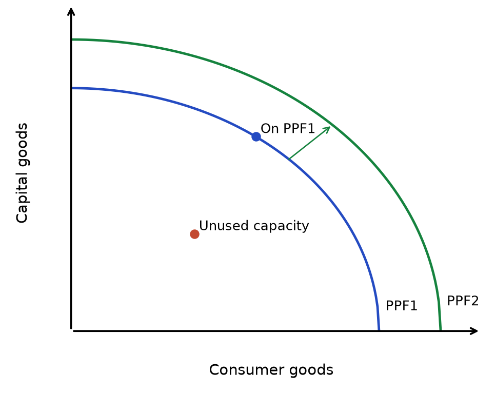
Read the diagram: A point inside the frontier uses resources inefficiently. Moving towards the existing frontier raises actual output; an outward shift increases productive potential. Moving along a bowed frontier involves increasing opportunity cost.
Assumptions: resources and technology are fixed for one frontier. A movement along it reallocates resources; moving towards it uses idle resources; shifting it changes productive capacity.
Comparing GDP/GNI between countries and over time (spec point d): When comparing economic performance across countries or across time periods, always check:
- Are figures real or nominal? Nominal figures are distorted by inflation — always use real GDP for comparison
- Are figures total or per capita? Total GDP tells you the size of the economy; per capita tells you average living standards — a country with high total GDP but large population may have low living standards per person
- Have PPP adjustments been applied? Without PPP, cost-of-living differences distort cross-country comparisons
- Is the data reliable? Developing countries may have large informal sectors or weak statistical collection
Limitations of GDP/GNI as a measure of living standards
- This is a frequently tested exam topic — examiners want a specific mechanism and consequence for each limitation, not just a vague statement.
Quality changes are difficult to measure
Mechanism: Statistical agencies adjust prices for changes in quality, but separating improved quality from inflation is difficult, especially for rapidly changing products.
Exam-focused consequence: Incomplete quality adjustment can distort measured real growth. GDP may not fully capture the welfare gain from better technology, even when some improvement is included.
Unpaid services and informal production
Mechanism: Unpaid household services such as cleaning and childcare are normally outside GDP. Goods produced for own use, including subsistence crops, and informal market production are conceptually included, but may be difficult to estimate.
Exam-focused consequence: Different measurement coverage can distort comparisons. A shift from unpaid household childcare to paid childcare can raise measured GDP without an equivalent increase in services received.
Hidden/black market economy
Mechanism: National accounts can include estimates of concealed and illegal market production, but these activities are difficult to observe and may be under-recorded.
Exam-focused consequence: Incomplete estimates of the shadow economy can understate output. Differences in statistical coverage make comparisons less reliable.
Income distribution ignored
Mechanism: GDP per capita is an average — it divides total output by population without showing how income is spread
Exam-focused consequence: Two countries can have identical GDP per capita but very different living standards if one has high inequality (a small rich elite) and the other has a more even distribution
Externalities of growth not deducted
Mechanism: GDP only counts the value of output, not the costs imposed on third parties in producing it
Exam-focused consequence: Growth driven by heavy industry may come with pollution, congestion, and longer working hours — GDP rises even as quality of life for some falls
No measure of wellbeing/happiness
Mechanism: GDP is a purely monetary measure and cannot capture non-material aspects of welfare
Exam-focused consequence: Higher income does not guarantee higher life satisfaction beyond a certain point (see Easterlin paradox below) — GDP growth may overstate true welfare gains
→ Because of these limitations, examiners expect you to suggest an alternative or supplementary measure (e.g. Human Development Index, Gross National Happiness, inequality-adjusted HDI) when asked to evaluate GDP as a measure of living standards, rather than simply listing its flaws.
National happiness and wellbeing
- As a response to the limitations of GDP, some economists and governments have shifted toward measuring national happiness directly, rather than relying solely on monetary output.
Gross National Happiness (Bhutan) — an alternative measure of national progress based on non-economic criteria, including:
Psychological wellbeing
Health
Education
Time use
Cultural diversity and resilience
Good governance
Community vitality
Ecological diversity and resilience
Living standards
The Easterlin paradox refers to the finding that, although higher-income people often report greater happiness within a country, rising average income over time does not necessarily produce a corresponding sustained rise in average reported happiness. This is a debated empirical relationship, not a universal income threshold.
Why this happens (exam explanation):
→ Once basic needs (food, shelter, security) are met, additional income satisfies fewer pressing needs → marginal utility of extra income falls
→ People care about relative income (their income compared to others), not just absolute income → if everyone's income rises together, relative position — and therefore happiness — may not improve
→ Higher income is often accompanied by longer working hours, more stress, and less leisure time → these offset some of the wellbeing gains from higher income
Exam application: higher real income can improve material living standards, but changes in inequality, health, leisure, relationships and environmental quality also matter. Avoid claiming that growth is necessary for every improvement in wellbeing or that happiness stops rising at one universal income level.
Section recap: Use real GDP for output growth, per-capita values for average output, and PPPs for cross-country purchasing-power comparisons. Add distributional and non-material indicators when judging living standards.
Inflation
Inflation — a sustained increase in the general price level over time, reducing the purchasing power of money.
Deflation — a sustained decrease in the general price level.
Disinflation — a fall in the rate at which the general price level is rising (prices are still going up, but more slowly).
Measuring inflation: Consumer Price Index (CPI)
CPI (Consumer Price Index) — a measure of the average change in prices of a representative basket of goods and services purchased by households, used to calculate the rate of inflation.
How CPI is calculated:
- Household expenditure data identify spending patterns used to select the basket and calculate expenditure weights; methods and coverage vary between countries.
- A weighted basket of goods and services is created (e.g. petrol has a higher weight than tea)
Prices are collected monthly from various locations
The basket and weights are updated annually to reflect changing spending patterns
A base year is chosen (index = 100) for comparison
Annual inflation rate = ((CPI this year − CPI previous year) ÷ CPI previous year) × 100. For a monthly index, year-on-year inflation compares the month with the same month one year earlier; the index reference year is not automatically the comparison period.
Worked example: CPI rises from 125 to 130 over one year. Annual inflation = (130 − 125) ÷ 125 × 100 = 4%. The index being 130 means prices are 30% above the reference-year level, not that this year’s inflation is 30%.
Limitations of CPI
| Limitation | Explanation |
|---|---|
| Representative basket | Only reflects the "average" household — not accurate for non-car owners, renters, etc. |
| Quality changes | Hard to separate price rises from quality improvements (e.g. a better phone at a higher price) |
| New technology | Slow to include new products; hard to make historical comparisons |
| Housing costs | CPI does not fully capture housing costs (mortgage interest, council tax) — RPI includes these |
Definition reminder: RPI (Retail Price Index)
- RPI tends to be higher than CPI.
Producer (Wholesale) Price Index (PPI) — measures the average change in prices charged by domestic producers for their output.
- Used as a leading indicator of future consumer price inflation.
Causes of inflation
| Type | Source | Mechanism | Examples |
|---|---|---|---|
| Demand-pull | AD side | AD rises → excess demand at current prices → producers raise prices | ↓ interest rates → ↑ C and I → ↑ AD → ↑ PL; fiscal stimulus (↓ tax → ↑ disposable income → ↑ C); depreciation (↑ exports, ↓ imports → ↑ net X) |
| Cost-push | AS side | Costs of production ↑ → SRAS shifts left → ↑ PL | ↑ oil/commodity prices; ↑ wages (trade unions); ↑ indirect taxes; depreciation (↑ import costs) |
| Money supply growth | Monetary side | Monetary expansion may raise spending and AD; the price-level response depends on spare capacity and the response of output. | QE → lower yields and easier financial conditions → potentially ↑ spending and AD → upward pressure on PL, depending on spare capacity |
Figure 2.2 AD and AS equilibrium
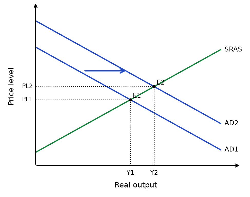
Read the diagram: Identify a non-price determinant that changes AD → shift AD right, holding the other curve fixed → find the new intersection → price level rises and real output rises. The price-level change is a movement along the unchanged curve. This result assumes upward-sloping SRAS; spare capacity and the curve’s slope determine the real-output response. A higher price level is not the same as a permanently higher inflation rate.
Figure 2.3 AD and AS equilibrium
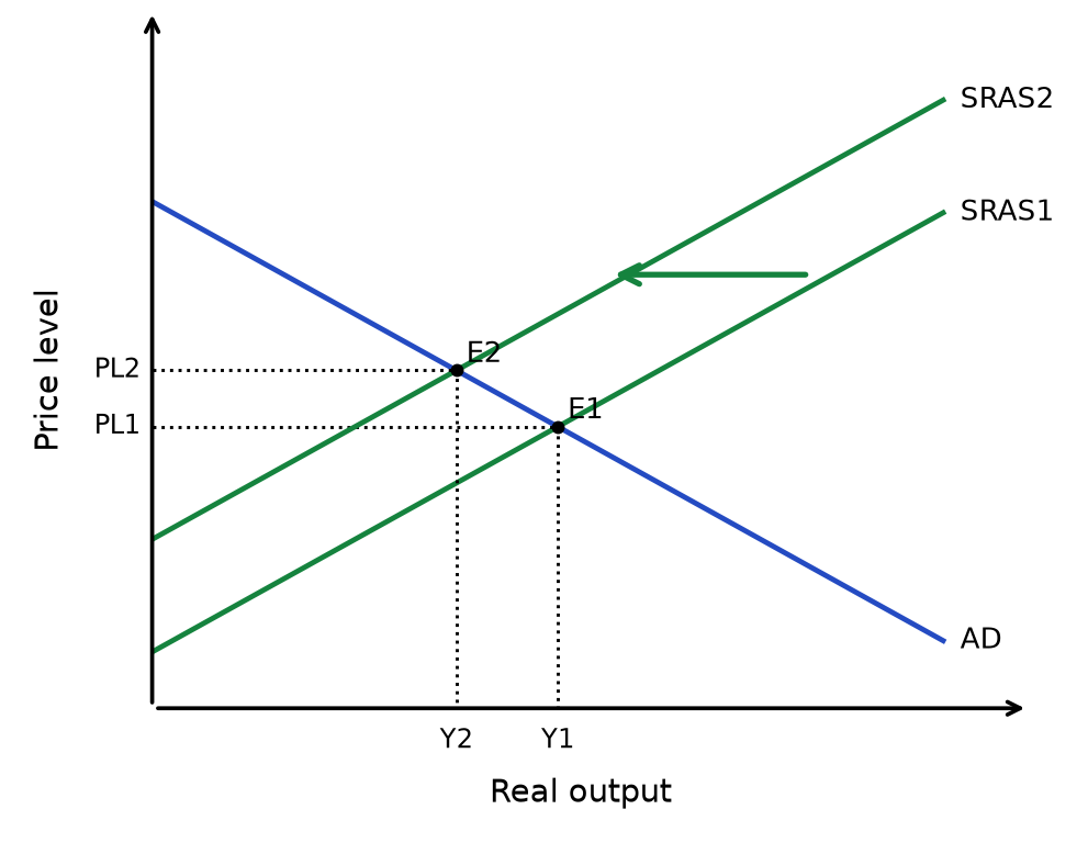
Read the diagram: Identify a non-price determinant that changes SRAS → shift SRAS left, holding the other curve fixed → find the new intersection → price level rises and real output falls. The price-level change is a movement along the unchanged curve. This result assumes upward-sloping SRAS; spare capacity and the curve’s slope determine the real-output response. A higher price level is not the same as a permanently higher inflation rate.
Exam tip — how to tell them apart in a data response:
↑ price level and ↑ real GDP are consistent with an increase in AD when SRAS is unchanged. They do not alone prove the cause: use the extract to identify the spending change and consider simultaneous supply shifts.
↑ price level and ↓ real GDP are consistent with an adverse SRAS shift when AD is unchanged. Check the evidence for higher costs or disrupted production before attributing the outcome to cost-push inflation.
Policy depends on the source of inflation. Demand restraint addresses excessive spending; supply measures may address production constraints. With combined shocks, assess the trade-off between reducing inflation and supporting output.
Causes of deflation
- Fall in AD (e.g. cut in government spending → ↓ C and G → ↓ AD → ↓ PL)
- Increase in AS (e.g. ↑ productivity → ↑ SRAS → ↓ PL)
Decrease in money supply
Effects of inflation (detailed, exam-focused)
Consumers:
→ Inflation ↑ → if nominal income doesn't rise as fast → real income and purchasing power ↓ → consumers can buy fewer goods and services → standard of living falls
Effect is regressive
low-income households spend a larger share of income on necessities (food, energy) whose prices often rise fastest → low-income households hit hardest
People whose nominal incomes fail to keep pace with their living costs lose purchasing power. Some pensions and benefits are uprated, although delays and differences in household spending patterns can leave recipients exposed.
Real value of savings falls (money saved today buys less in the future) → discourages saving, may encourage riskier spending or borrowing behaviour
Firms:
→ Inflation creates uncertainty about future costs and prices → firms find it harder to plan and forecast → business confidence ↓ → investment (I) ↓ → AD and future productive capacity ↓
Rising costs (wages, raw materials) squeeze profit margins unless firms can pass costs on via higher prices
If domestic inflation is higher than trading partners' → domestic goods become relatively more expensive → international price competitiveness ↓ → exports ↓, imports ↑ → current account may worsen
Menu costs
firms must frequently update prices (menus, price tags, contracts), which is administratively costly
Workers:
→ If nominal wage growth < inflation → real wages ↓ → workers effectively take a pay cut in terms of purchasing power → may prompt wage demands or industrial action
Wage-price spiral risk
workers demand higher wages to keep up with inflation → firms' costs ↑ → firms raise prices further → inflation persists or accelerates
Government:
Inflation can push taxpayers into higher tax brackets without a real increase in income (fiscal drag) → government tax revenue ↑ in nominal terms
Government spending on benefits/pensions linked to inflation (index-linked) must rise to maintain real value → government expenditure ↑ → pressure on the budget
Real value of government debt falls with inflation (debt is often fixed in nominal terms) — a benefit for a government carrying large debt, but a real loss to bondholders
Savers and borrowers:
Savers lose
fixed nominal savings become worth less in real terms as prices rise → real return on savings falls, and may become negative if inflation exceeds the interest rate
Borrowers gain
the real value of a fixed nominal debt falls as inflation erodes it → effectively cheaper to repay debt in real terms
International competitiveness / balance of payments:
Domestic inflation higher than trading partners → relative price of exports ↑, relative price of imports ↓ (in the eyes of foreign/domestic buyers) → exports ↓, imports ↑ → net exports fall → current account deficit worsens
Effects of deflation (detailed, exam-focused)
Consumers:
→ Falling prices ↑ real purchasing power of a given income → in principle, consumers can buy more → BUT if consumers expect prices to fall further → they delay purchases waiting for a better price → consumer spending (C) ↓ → AD ↓ — this is the key exam point about deflation
Firms:
→ ↓ AD → firms' revenues and profits fall → firms may cut back on investment, wages, or staff to reduce costs → can trigger redundancies and rising unemployment
Deflationary spiral risk
falling AD → firms cut prices/output/jobs → unemployment ↑ → incomes fall further → AD falls further → deepens the deflation
Debt burden:
→ If prices fall but nominal debts are fixed → the real value of debt rises → firms and households with debt face a heavier real repayment burden → may cut spending further to service debt, or default → risk of bankruptcies
Government:
→ ↓ nominal incomes and spending → tax revenue (income tax, VAT) ↓
Real value of government debt ↑ (same mechanism as private debt) → harder to manage public finances
International competitiveness:
Domestic prices falling relative to trading partners → exports become relatively cheaper, imports relatively dearer → exports ↑, imports ↓ → current account improves — this is one of the few "benefits" of deflation, but is usually outweighed by the domestic costs of falling AD and rising unemployment
Phillips curve (short run) — suggests an inverse relationship between inflation and unemployment: when AD rises, inflation ↑ and unemployment ↓; when AD falls, inflation ↓ and unemployment ↑.
This illustrates a possible short-run conflict between low inflation and low unemployment. The relationship depends on the source of the shock; rising production costs can raise inflation and unemployment together.
Macroeconomic objectives and possible conflicts
The six objectives are economic growth; low and stable inflation; low unemployment; equilibrium on the current account; a balanced government budget; and greater income equality. Governments may give these different weights depending on the economy’s circumstances.
Inflation and unemployment: with spare capacity and stable expectations, higher AD may raise employment but also increase inflationary pressure. A supply shock can worsen both outcomes, so there is no guaranteed stable trade-off.
Growth and environmental protection: higher output can increase pollution and resource depletion; cleaner technology and environmental regulation may reduce the conflict, although implementation has costs.
Inflation and current-account equilibrium: higher domestic inflation relative to trading partners can weaken price competitiveness, reduce exports and increase imports, other things equal. Exchange rates, demand elasticities and non-price competitiveness affect the result.
Growth and income equality: growth concentrated in skilled employment or asset ownership may widen inequality; wider access to education, employment and redistribution can spread the gains. Growth does not automatically make income distribution more or less equal.
Figure 2.4 Short-run Phillips curve
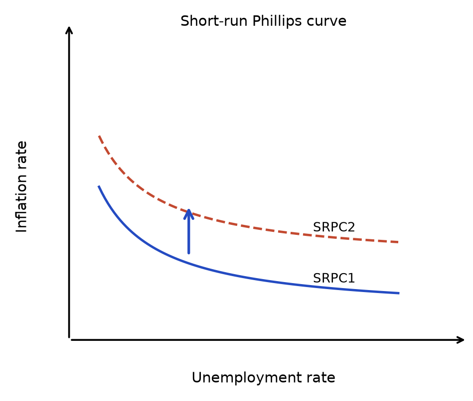
Read the diagram: A movement along SRPC1 illustrates a possible short-run AD-related trade-off, holding other influences constant. An adverse supply shock can shift the relationship outward, allowing inflation and unemployment to rise together.
Section recap: Inflation is a sustained price-level increase; disinflation is slower inflation and deflation is a falling price level. Annual CPI inflation compares the index with a year earlier.
Employment and Unemployment
Unemployment — people without work who sought work in the previous four weeks and can start within two weeks; also those without work who have a job arranged to start within two weeks.
Underemployment — people who have a job but whose labour is not fully utilised (e.g. part-time workers who want full-time work, or workers in jobs below their skill level).
Economically inactive — outside employment and not actively seeking work and/or unavailable to start. Examples may include students, carers, retirees and discouraged workers; classify people by their activity and availability, not their label alone. UK statistics often report a 16–64 age band.
Calculating employment, unemployment and inactivity rates
The three rates use different denominators. Employment and inactivity rates compare people with the relevant population; the unemployment rate compares unemployed people with the labour force. The labour force is employed people plus unemployed people.
| Measure | Calculation |
|---|---|
| Employment rate | Employed ÷ population in the stated age group × 100 |
| Unemployment rate | Unemployed ÷ (employed + unemployed) × 100 |
| Inactivity rate | Economically inactive ÷ population in the stated age group × 100 |
Use the age group given in the data. UK headline employment and inactivity rates usually refer to ages 16–64, while the headline unemployment rate refers to the economically active population aged 16 and over. The hypothetical example below uses the same age group throughout so the denominators can be compared directly.
Worked example: more people enter the labour force
In a hypothetical population of 1,000 people of the same stated age group, 30 previously inactive people begin participating in the labour market. Twenty find jobs and ten are available for work and actively looking for it. There are no other changes.
| Labour-market status | Period A | Period B |
|---|---|---|
| Employed | 600 | 620 |
| Unemployed | 50 | 60 |
| Economically inactive | 350 | 320 |
| Total population | 1,000 | 1,000 |
| Labour force | 650 | 680 |
Calculate the three rates for each period. Does a higher unemployment rate necessarily mean fewer people have jobs?
| Rate | Period A | Period B |
|---|---|---|
| Employment | 600 ÷ 1,000 × 100 = 60% | 620 ÷ 1,000 × 100 = 62% |
| Unemployment | 50 ÷ 650 × 100 ≈ 7.69% | 60 ÷ 680 × 100 ≈ 8.82% |
| Inactivity | 350 ÷ 1,000 × 100 = 35% | 320 ÷ 1,000 × 100 = 32% |
Employment rises by 20 people and its rate rises by 2 percentage points. Unemployment also rises: ten new labour-force participants have not yet found work. Its rate increases by approximately 1.13 percentage points, while inactivity falls by 3 percentage points.
A higher unemployment rate therefore does not necessarily mean employment has fallen. Check flows into and out of the labour force as well as the numbers in work.
Common mistake: these three rates do not sum to 100%, because unemployment has a different denominator. With a common age group, the employment rate and inactivity rate sum to less than 100%; the remaining population share is unemployed people divided by that population, not the unemployment rate.
Types of unemployment overview
| Type | Cause | Key mechanism | Duration / severity |
|---|---|---|---|
| Cyclical (demand-deficient) | ↓ AD during recession | ↓ consumer spending → firms cut output → redundancies | Linked to business cycle; rises in recessions |
| Structural | Long-term decline in an industry, worsened by factor immobility | Industry loses competitiveness → jobs disappear permanently → workers cannot easily move to new jobs | Long-term / persistent |
| Frictional | Time between leaving one job and starting another | Workers searching for the right job match | Usually short-term; job matching can improve, but lost income and forgone output still impose costs. |
| Seasonal | Seasonal variation in demand | Tourism, agriculture, retail hire in peak seasons, lay off in off-seasons | Predictable; returns each year |
| Real wage (classical) | Wages kept above equilibrium | Wage > market-clearing level (e.g. NMW, trade unions) → supply of labour > demand | Persistent until wages adjust |
Figure 2.5 Minimum wage
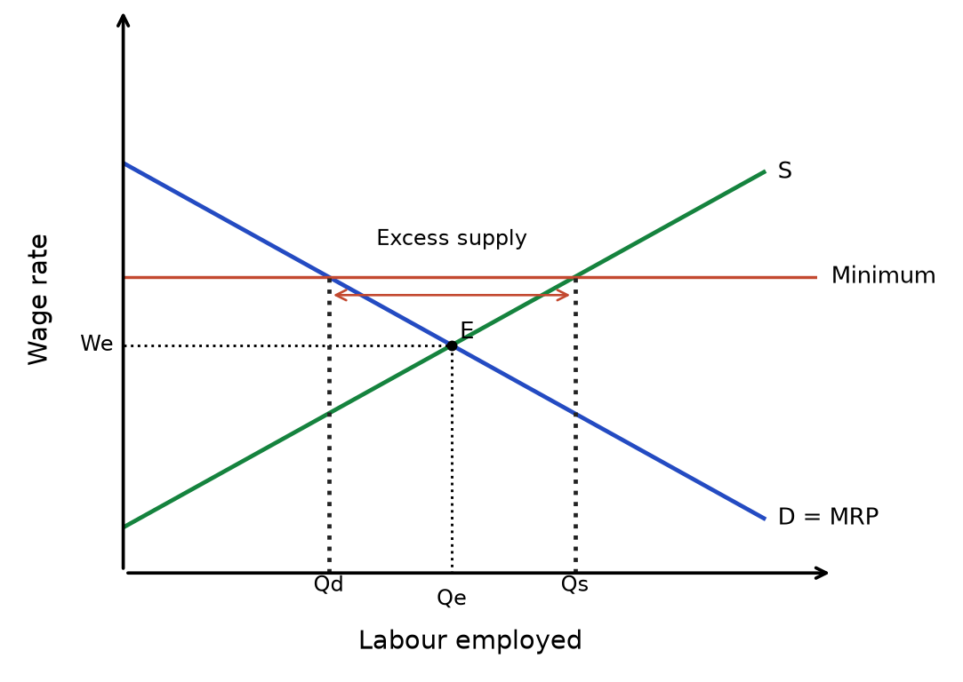
Read the diagram: A binding floor above equilibrium makes quantity supplied exceed quantity demanded. The gap is excess supply. This is the competitive labour-market model; a monopsony requires a different analysis.
Cyclical (demand-deficient) unemployment
Cyclical unemployment — unemployment caused by a fall in aggregate demand during a recession or economic downturn, when firms cut back on production and lay off workers.
Mechanism:
→ A fall in AD reduces demand for firms’ output → firms cut production and employment → household incomes and consumption fall → the multiplier can deepen the initial downturn.
Link to the output gap:
A negative output gap means actual GDP is below potential GDP. Recession concerns falling output, not its level relative to potential. A recovery can reduce cyclical unemployment while output remains below potential.
Examples:
- The 2008 financial crisis → ↓ AD → firms across construction, retail, manufacturing made mass redundancies
- COVID-19 pandemic → lockdowns → hospitality, travel, retail sectors cut staff
Why it matters for exams:
Demand stimulus directly addresses deficient spending. Explain why fiscal or monetary expansion can raise employment when there is spare capacity, then assess confidence, leakages and policy lags.
This distinction is a common exam evaluation point
Retraining alone does not create sufficient demand for labour. However, public training or infrastructure spending can also raise AD, and supply-side measures can limit persistent skill loss; the appropriate policy mix depends on the cause and duration of unemployment.
Structural unemployment
Structural unemployment — unemployment caused by a long-term decline in demand for goods and services in a particular industry or region, leaving workers without the skills or location needed for jobs elsewhere in the economy.
The core cause
structural unemployment persists specifically because of factor immobility — workers cannot easily move from a declining industry into a growing one. This is why it is one of the most persistent and damaging forms of unemployment.
Occupational immobility — workers lack the skills required to move from a declining industry into a growing one.
→ Industry declines (e.g. coal mining, shipbuilding, manufacturing) due to technological change or foreign competition → workers made redundant have industry-specific skills (e.g. mining, welding) that don't transfer to growing sectors (e.g. tech, services) → workers cannot retrain quickly or affordably → remain unemployed long-term despite job vacancies existing elsewhere in the economy
Causes of occupational immobility:
Lack of transferable skills (skills specific to the declining industry)
Insufficient education/training opportunities or funding to retrain
Age discrimination — older workers seen as less adaptable or worth retraining
Trade union restrictions or lack of information about retraining paths
Geographical immobility — workers are unable or unwilling to move location to take up jobs in areas of the country (or world) where they are available.
→ Jobs disappear in one region (e.g. a former industrial town) while vacancies exist in another (e.g. a growing city) → workers face barriers to relocating → unemployment persists in the declining region even as labour shortages exist elsewhere
Causes of geographical immobility:
High cost of housing in areas with job vacancies (regional house price differences)
Family and social ties (children's schooling, family care responsibilities)
Lack of affordable transport/commuting infrastructure between regions
Imperfect information about job vacancies in other areas
Why this matters for exam evaluation: when explaining structural unemployment, always link it explicitly to which type of immobility is at play, because this determines the appropriate policy response:
→ Occupational immobility as the cause → appropriate policy is retraining schemes / subsidised education → addresses the skills mismatch directly
→ Geographical immobility as the cause → appropriate policy is relocation subsidies / affordable housing / improved transport links → addresses the mobility barrier directly
→ Using the wrong policy (e.g. retraining when the real barrier is housing costs) means the intervention fails to reduce unemployment — this is a strong evaluative point
Consequences of structural unemployment:
Long-term / persistent — workers may remain unemployed for years, unlike frictional unemployment
Hysteresis effect
the longer someone is unemployed, the more their skills atrophy and the harder it becomes to find work — unemployment becomes self-reinforcing
Regional inequality — declining industries are often concentrated in specific regions, leading to persistent regional unemployment "black spots"
High cost to government — long-term claimants require sustained benefit payments and lost tax revenue over many years
Frictional unemployment
Frictional unemployment — short-term unemployment that occurs when workers are between jobs, i.e. the time lag between leaving one job and starting another while searching for a suitable match.
Why frictional unemployment exists — the exam explanation:
→ Labour markets have imperfect information — workers do not instantly know which firms are hiring, and firms do not instantly know which workers are available and suitable → a time-consuming search and matching process is required on both sides
→ Workers voluntarily leave jobs (to find a better match, due to relocation, or after graduating) and take time to find a new one that matches their skills, preferences and pay expectations → during this search period, they are counted as unemployed even though they will find work
Concrete examples to use in exam answers:
- A graduate leaving university and taking a few months to find a graduate-level job
- A worker resigning from one job to search for a better-paid or better-matched role elsewhere
- Someone relocating to a new city and needing time to find local employment
Why it is considered "less damaging" than other types:
- It is usually short-term: unemployment ends when a suitable job match is found, but the search may take longer if information or vacancies are limited.
- It reflects a healthy, dynamic labour market with worker choice and mobility, rather than a structural weakness in the economy
- Some frictional unemployment is inevitable and even desirable — it allows better job matching (higher productivity in the long run) rather than workers accepting the first available job
Why frictional unemployment can never be reduced to zero:
→ As long as some workers change jobs, resign, graduate, or relocate → there will always be a pool of people in the search-and-match process at any point in time → it is therefore impossible, and not necessarily desirable, to achieve 0% unemployment
Policy implications
Because frictional unemployment arises during job search and matching, improved information — e.g. job centres, online job matching platforms and careers advice — directly addresses the problem. Demand-side stimulus mainly addresses cyclical unemployment, while retraining addresses skills mismatch; these causes can coexist.
Seasonal unemployment
Seasonal unemployment — unemployment caused by regular, predictable fluctuations in demand for labour at certain times of the year, linked to seasonal patterns in specific industries.
Mechanism:
→ Certain industries experience ↑ demand during particular seasons and ↓ demand during others → firms hire more workers in peak seasons and lay them off in off-seasons → workers in these industries face predictable periods of unemployment each year
Examples:
- Tourism and hospitality → ↑ employment in summer holidays, ↓ in winter
- Agriculture → ↑ employment during harvest, ↓ during off-season
- Retail → ↑ employment before Christmas, ↓ in January
- Construction → ↓ employment during winter months due to weather
Why it differs from other types:
- It is predictable — workers and firms know when employment will rise and fall
- It is temporary and recurring — the same workers may be rehired each peak season
- Workers can sometimes plan around it (e.g. take a different job in the off-season)
Why it matters for exams:
Seasonal unemployment reflects predictable changes in labour demand. General demand stimulus may not remove these patterns. Retraining, mobility support, diversification and extending the tourist season can reduce them; these can be supply-side measures. Temporary income support cushions lost earnings but does not itself create year-round jobs.
Real wage (classical) unemployment
Real wage unemployment — unemployment caused when the real wage rate is maintained above the market-clearing equilibrium level, so that the supply of labour exceeds the demand for labour.
Mechanism:
→ Wages are set above the equilibrium wage (W_e) → at this higher wage, more people are willing to work (↑ quantity of labour supplied) but firms want to hire fewer workers (↓ quantity of labour demanded) → supply of labour > demand for labour → the gap (Q_s − Q_d) = real wage unemployment
Causes of wages being above equilibrium:
- National Minimum Wage (NMW) — government sets a legal floor below which wages cannot fall; if NMW > W_e, unemployment is created
- Trade union power — unions collectively bargain for wages above the market-clearing level
- Efficiency wage theory — firms voluntarily pay above-equilibrium wages to boost worker morale, reduce turnover, and increase productivity (the productivity gain may offset some or all of the higher wage cost)
Diagram link: Minimum wage earlier in this topic. Apply the same labels and assumptions to the change described here.
The classical economist argument:
→ If wages were perfectly flexible, they would fall to W_e and unemployment would disappear → classical economists argue that labour market rigidities (NMW, unions) prevent this adjustment → removing these rigidities would eliminate real wage unemployment
Evaluation (the counter-argument examiners expect):
→ Cutting wages during a downturn would ↓ disposable income → ↓ consumer spending (C) → ↓ AD → could worsen cyclical unemployment and push the economy into recession
- The classical argument assumes a perfectly competitive labour market, which is unrealistic — in practice, labour markets have imperfect information, monopsony power, and bargaining asymmetries
- NMW may actually increase employment in a monopsony (where a single employer has wage-setting power and would otherwise pay below W_e) — so the effect of NMW on unemployment depends on market structure
Common mistake: don't assume cutting the minimum wage always reduces unemployment — in a monopsony labour market the effect can run the opposite way, so market structure must be considered before concluding.
Policy implications
reducing real wage unemployment requires either lowering the minimum wage (politically difficult and risks poverty), weakening union power (may worsen inequality), or improving labour market flexibility — but each has significant trade-offs.
Summary: matching policy responses to unemployment type
- This table is the key exam tool — always identify the type of unemployment first, then match the correct policy. Using the wrong policy is a common exam evaluation point.
| Type | Root cause | Appropriate policy response | Limit or qualification |
|---|---|---|---|
| Cyclical | ↓ AD | Demand-side: ↑ G, ↓ taxes, ↓ interest rates (↑ AD) | Retraining alone does not address deficient spending; policy spending may also raise AD. |
| Structural (occupational) | Skills mismatch | Supply-side: retraining, education, apprenticeships | Demand stimulus alone does not remove skills mismatch; training and spending that supports new employment may complement it. |
| Structural (geographical) | Location barriers | Supply-side: relocation subsidies, affordable housing, transport links | Retraining alone may be insufficient where location barriers remain; training for accessible jobs can still help. |
| Frictional | Imperfect information | Improve information: job centres, online platforms, careers advice | Better matching is the direct response; demand support may also be relevant if weak demand coexists. |
| Seasonal | Seasonal demand patterns | Economic diversification, temporary income support | Demand-side stimulus can't change seasonal demand patterns |
| Real wage | Wage > equilibrium | Reduce NMW / weaken unions (but with significant trade-offs) | Training may raise productivity and labour demand, but does not directly remove a wage floor above equilibrium. |
Common mistake: match policy to the cause. Demand stimulus directly addresses weak aggregate demand; retraining, mobility and job-search support address skills or matching problems. Policies can complement each other, and diversification can reduce seasonal unemployment.
Unemployment vs underemployment
- Although related, unemployment and underemployment measure different problems in the labour market, and it is a common exam point that the two can move in opposite directions.
| Unemployment | Underemployment | |
|---|---|---|
| Definition | People without any job who are available and actively seeking work | People who have a job, but whose labour is not used to its full potential |
| ILO status | Counted as unemployed | Counted as employed (has a job) — NOT captured by the unemployment rate |
| Examples | Made redundant and searching for work; graduate who has never worked | Part-time worker who wants full-time hours; graduate working in a low-skill job below their qualification level; worker on a zero-hours contract wanting more hours |
| What it reflects | A complete lack of employment | Employment that fails to fully use a worker's skills, qualifications, or desired hours |
| Effect on GDP | Lost output entirely from those not working | Output is produced, but below the worker's full productive potential — a hidden loss of potential output |
| Measurement issue | Directly captured by the ILO unemployment rate | NOT captured by the headline unemployment rate — a country can have low unemployment but high underemployment, giving a misleadingly rosy picture of the labour market |
Why this distinction matters for exams:
→ A falling unemployment rate does not necessarily mean the labour market is healthy → if much of the "employment" is underemployment (involuntary part-time work, workers overqualified for their jobs) → living standards and productivity may still be below potential → headline unemployment statistics can overstate labour market strength
Common mistake: don't treat a falling headline unemployment rate as automatic proof of a healthy labour market — always consider whether it has been accompanied by rising underemployment, which would undermine the positive interpretation. This is a strong evaluative point when discussing "the significance of changes in the unemployment rate."
Effects of unemployment
| Group | Effects |
|---|---|
| Individuals | ↓ disposable income → ↓ living standards; psychological effects (loss of confidence, mental health); skills erosion if long-term |
| Firms | ↓ sales and revenue (less consumer spending); but larger pool of labour to hire from → ↓ wage pressure |
| Government | ↓ income tax revenue + ↓ VAT revenue (less spending); ↑ spending on unemployment benefits → opportunity cost |
| Society | Opportunity cost of lost output (goods/services the unemployed could have produced); ↑ crime, social unrest |
| Economy | Lower income can reduce C and AD through the multiplier. Initially, actual output lies inside the PPF; prolonged unemployment may also damage skills and investment, reducing future productive potential. |
Net migration and the labour market
Net migration: immigration minus emigration over a stated period.
| Effect | Mechanism |
|---|---|
| ↑ labour supply | Migrants are usually of working age → S_L shifts right → ↓ wages (if demand unchanged) |
| ↑ competition for jobs | More job seekers → some domestic workers may be displaced |
| Skills and productivity | Migrants may bring skills in shortage areas → ↑ productivity → ↑ productive potential |
| Fiscal contribution | Working migrants pay taxes → ↑ government revenue; less likely to claim benefits in short term |
| Net effect | Depends on skill level — high-skilled migrants tend to boost productivity and growth; low-skilled may add to labour supply without displacing existing workers |
Section recap: Unemployment excludes people outside the labour force. Distinguish its causes from underemployment, and select policies that address the relevant demand, skills, location or wage problem.
Balance of Payments
Balance of payments — a record of economic transactions between residents of an economy and non-residents over a given period.
- The balance of payments has three accounts, but the IAL spec focuses on the current account:
| Account | Records |
|---|---|
| Current account | Trade in goods and services, primary income and secondary income |
| Capital account | Capital transfers (e.g. debt forgiveness, asset transfers) |
| Financial account | Financial assets and liabilities (e.g. FDI, portfolio investment) |
Components of the current account
| Component | What it records | Example |
|---|---|---|
| Trade in goods (visible trade) | Exports and imports of physical goods | UK exports cars, imports electronics |
| Trade in services (invisible trade) | Exports and imports of services | UK exports financial services, imports tourism |
| Primary income | Income receivable from non-residents minus income payable to non-residents, including investment income and compensation of employees | UK residents earn dividends from overseas investments |
| International transfers (secondary income) | Transfers between countries | EU membership contributions, foreign aid, remittances |
Definition reminder: Current account deficit
- Current-account payments to non-residents exceed current-account receipts from non-residents.
Definition reminder: Current account surplus
- Current-account receipts from non-residents exceed current-account payments to non-residents.
Causes of current account imbalances
| Cause | Effect on current account | Mechanism |
|---|---|---|
| Exchange rate appreciation | May worsen the balance | Appreciation may raise foreign-currency export prices and lower domestic-currency import prices. The effect on trade values depends on price elasticities and pass-through. |
| Economic growth | May worsen the balance | ↑ GDP → ↑ disposable income → ↑ M (high marginal propensity to import) → deficit worsens |
| International competitiveness | May improve the balance | ↓ inflation relative to trading partners → exports cheaper → ↑ X, ↓ M → deficit improves |
| Deindustrialisation | May worsen the balance | Manufacturing declines → goods previously made domestically now imported → ↑ M |
| Productivity | May improve the balance | ↑ productivity → ↓ unit costs → exports more competitive → ↑ X |
Significance of current account imbalances
Deficit — why it matters (exam explanation):
A persistent current-account deficit requires net financing from abroad, allowing for the capital account and errors and omissions. Borrowing or selling assets can create future interest, dividend or profit payments abroad, which may make the deficit harder to finance. A current-account deficit need not imply a goods-and-services trade deficit.
→ Persistent deficit → foreign investors may lose confidence in the country's ability to repay → ↓ demand for the domestic currency → currency depreciates → imports become more expensive → cost-push inflation → ↑ SRAS costs → ↓ economic growth
A deficit financing productive capital imports may support future output and export earnings. This can improve sustainability, but only if investment is productive and financing remains affordable; the deficit is not automatically temporary or self-correcting.
Surplus — why it matters (exam explanation):
A persistent current-account surplus corresponds broadly to net lending abroad, allowing for the capital account. If it is driven by strong export demand, upward pressure on the currency may weaken price competitiveness and narrow the trade surplus, depending on the exchange-rate regime and other capital flows.
→ Surplus may indicate that domestic consumption and investment are too low → the country is producing for foreign consumers rather than its own citizens → living standards may be lower than they need to be
→ Trade partners running deficits against this country may become frustrated → may impose tariffs or protectionist measures → ↓ exports → surplus narrows (e.g. US-China trade tensions)
Exam evaluation — is a current account deficit always a problem?
| Factor | Indicators of greater financing risk | Indicators of greater sustainability |
|---|---|---|
| Composition of imports | Importing consumer goods (consumption-led) | Importing capital goods (investment-led) |
| Duration | Persistent, structural deficit | Temporary, cyclical deficit |
| Financing | Financed by short-term borrowing (hot money flows) | Financed by long-term FDI |
| Size | Large relative to GDP; assess context | Small relative to GDP; assess context |
| Economic context | Economy at full capacity (inflationary) | Economy in recession (demand-deficient) |
→ Use this table to build an evaluation: "A current account deficit is not necessarily a problem if it is temporary, small, and driven by importing capital goods that will increase future productive capacity. However, if it is persistent, large, and financed by short-term borrowing, it risks a currency crisis and worsening future deficits."
Exam explanation stems: effects of inflation
Use these ready-made stems to explain the effects of inflation in exam answers:
Competitiveness
↑ inflation relative to trading partners → domestic goods become relatively more expensive → ↓ X and ↑ M → current account deficit worsens → ↓ AD → ↓ economic growth
Savings and investment
High and unpredictable inflation → ↓ business confidence → firms uncertain about future costs and revenues → ↓ investment (I) → ↓ AD → ↓ long-run growth
Real incomes
Nominal wages rise slower than inflation → ↓ real wages → ↓ purchasing power → ↓ consumer spending (C) → ↓ AD → ↓ economic growth
Income redistribution
Unexpected inflation can reduce the real value of fixed nominal debts and financial assets. Effects on inequality depend on asset and debt holdings, interest rates, wage adjustments and income indexation; pensioners are not uniformly on incomes that never rise.
Phillips curve trade-off
In the short run, ↑ AD → ↑ inflation but ↓ unemployment (Phillips curve). However, if inflation becomes entrenched → workers expect higher wages → ↑ costs → ↓ SRAS → ↑ unemployment (stagflation).
Exam explanation stems: unemployment
Use these ready-made stems to explain unemployment in exam answers:
Identifying the type
↓ AD during recession → firms cut output → redundancies → cyclical unemployment rises. This is distinct from structural unemployment (caused by factor immobility) and frictional unemployment (caused by imperfect information in job search).
Structural unemployment and immobility
Industry declines due to technological change/foreign competition → workers lack transferable skills (occupational immobility) or cannot relocate to where jobs exist (geographical immobility) → unemployment persists long-term → hysteresis effect worsens the problem as skills atrophy over time.
Why the policy must match the type
Cyclical unemployment → demand-side policy (↑ G, ↓ interest rates) to ↑ AD. Structural unemployment → supply-side policy (retraining, transport infrastructure). Demand stimulus alone does not remove skills or location barriers, but it can complement measures that improve matching and support new employment.
Unemployment and AD multiplier
↑ unemployment → ↓ disposable income → ↓ C → ↓ AD → firms cut further output → further redundancies → unemployment worsens (multiplier effect deepens the recession).
Falling unemployment may mask underemployment
Headline unemployment rate ↓ but many new jobs are part-time or below workers' skill levels → underemployment ↑ → productivity and living standards may not actually improve → unemployment statistics alone can overstate labour market health.
Exam explanation stems: economic growth and living standards
Use these ready-made stems to explain economic growth and evaluate GDP as a measure of living standards in exam answers:
GDP vs living standards
↑ real GDP does not automatically mean ↑ living standards → GDP per capita masks income inequality → the gains of growth may accrue to a small elite while most people see no improvement → use this to argue that GDP is a necessary but insufficient measure of welfare.
Nominal vs real
If nominal GDP rises by 5% but inflation is 3% → real GDP growth is approximately 2% (exactly 1.05 ÷ 1.03 − 1 = 1.94%, using the GDP deflator) → using nominal figures overstates actual economic performance → always adjust for inflation when comparing over time.
PPP in comparisons
Comparing GDP using market exchange rates ignores cost-of-living differences → $1 buys more in a low-cost country than a high-cost one → PPP-adjusted GDP provides a more accurate basis for comparing living standards between countries, especially developed vs developing.
GDP limitations — quality and informal economy
Quality improvements and informal production may be imperfectly measured, while unpaid household services are normally excluded → GDP may miss some welfare gains or output → evaluate measurement coverage alongside distribution and non-material living standards.
Easterlin paradox for evaluation
higher income is often associated with greater reported wellbeing within a country, but long-run income growth need not produce a matching increase in average happiness. Relative income, health, leisure and the environment also matter; there is no universal income cut-off.
Exam explanation stems: balance of payments
Use these ready-made stems to explain current account imbalances in exam answers:
Exchange rate and the current account
↑ exchange rate → exports may become more expensive for foreign buyers and imports cheaper for domestic buyers → export volumes may fall and import volumes rise. The effect on the current-account balance depends on price elasticities, pass-through and income flows. Depreciation can improve the trade balance under the standard Marshall–Lerner conditions, after time for volumes to adjust.
Economic growth and the current account
↑ GDP → ↑ disposable income → spending on imports may rise, especially with a high marginal propensity to import → downward pressure on the current-account balance, other things equal. Export growth and income flows may offset this effect.
Why a deficit may be self-reinforcing
A persistent deficit may be financed by borrowing or selling assets to non-residents. Future interest, dividend or profit payments can increase primary-income outflows and make the deficit harder to reduce; productive investment may also raise future income and exports.
Currency depreciation risk
A persistent deficit financed by volatile capital inflows can increase vulnerability to a loss of investor confidence. If those inflows reverse, downward pressure on the currency may raise import prices and production costs. A currency crisis is a risk, not an inevitable consequence of a deficit.
Evaluation — is a deficit always a problem? A small or temporary deficit driven by imports of productive capital goods may be sustainable. A large, persistent deficit financed by short-term borrowing is more vulnerable to a reversal of inflows. Assess the cause, financing, repayment capacity and likely future export earnings.
Section recap: The current account includes trade and primary and secondary income. Evaluate an imbalance using its cause, persistence and financing rather than its sign alone.
Assess several indicators together. Falling unemployment can reflect people leaving the labour force, while rising real GDP per head can hide unequal gains; check the underlying numbers and measurement limitations before judging performance.
Rapid recap
Growth: distinguish nominal from real GDP and total from per-person output; higher GDP per head does not show how gains are distributed.
Inflation: compare the rate of price increase over matching periods. Disinflation is slower price growth; deflation is a falling price level.
Employment: distinguish unemployment from inactivity and check the denominator. A lower unemployment rate need not mean more people are employed.
External balance: separate the current account from the fiscal balance. Judge growth, prices, jobs and external sustainability together, using measurement limitations where relevant.
Diagram cue: choose AD–AS, a PPF or a Phillips curve only when it supports the indicator being explained.
Related chapters: Unit 2 chapter 2 (p. 32) · Unit 2 chapter 6 (p. 70) · Unit 4 chapter 15