3.6 Demand management (demand-side policies) - fiscal policy
The government budget
As with any household (or firm), the government has its own income and expenditure.
Government income comes from:
- Indirect and direct taxes
- Sales of goods and services by state-owned enterprises
e.g. the income from the sale of stamps by the Hong Kong Post, a department of the Hong Kong government. - Privatising (selling of) state-owned enterprises
e.g. (partial) privatisation of the MTR Corporation in 2000 in Hong Kong.
Government expenditure can be classified into:
- Current expenditures
This includes wages to government employees, and purchases of goods of the consumption by the government. - Capital expenditures
Public investment spending, e.g. road and rail infrastructure. - Transfer payments
Government spending for which no good or service is provided in exchange, e.g. unemployment benefits, or agricultural subsidies provided by the EU.
Government expenditure can be financed by its income or by borrowing.
Budget deficit is when government expenditure is greater than government income. Debt might occur under a budget deficit situation.
Budget surplus is when government income is greater than government expenditure. The surplus can be used to pay off debts, or be used to accumulate savings.
Balanced budget is when government income is equal to government expenditure.
The goals of fiscal policy
The government might implement fiscal policy to achieve a range of economic goals:
- The maintenance of a low and stable rate of inflation.This can be achieved through managing government spending and taxation to keep AD stable.
- A low unemployment rate.
- A stable economic environment for long-term growth.
- Reducing fluctuations in the business cycle.
- Promoting an equitable distribution of income.
- Achieving an external balance between export revenue and import expenditure.
Expansionary and contractionary fiscal policies in order to close deflationary/recessionary and inflationary gaps
Fiscal policy is a demand-side policy using changes in government spending and/or taxation to shift the AD curve in order to achieve economic objectives.
As a large entity in the economy, government expenditure (G) and tax decisions (T) have a significant influence on the level of aggregate demand in the economy, and these can be used as policy tools to achieve macroeconomic goals.
At times, the output of the economy may fall below the potential level and a deflationary gap results. In such cases, the government may choose to use an expansionary fiscal policy, which can be in the form of:
(1) Increase in government expenditure
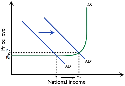
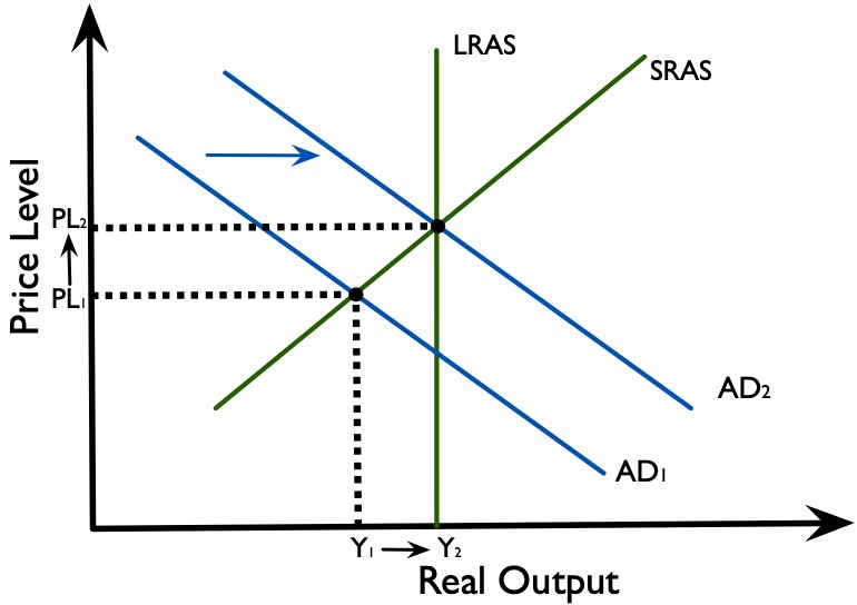
As government expenditure is a component of the AD, an increase in government expenditure will directly lead to an increase in AD. This is shown by the rightward shift of \(AD\) to \(AD’\) in Figure 3.6.1 and 3.6.2.
(2) Reduction of taxes
The effect of reducing taxes (T) is less direct in comparison to government spending (G). Tax reduction, e.g. income tax, increases households’ disposable income and encourages consumption (C). If the tax levied on firm profits is reduced, this increases the firms’ retained profit and may encourage investment (I). Both of them can increase AD.
In response to the economic crisis resulting from the coronavirus pandemic in 2020, many governments undertook expansionary fiscal policy to boost their economies and mitigate the changes of a deep recession.
The German government, for example, passed an emergency supplementary budget of €156 billion for 2020, including a €50 billion plan to provide direct grants to small businesses and the self-employed. Under this plan, companies with up to five employees will be eligible for a one-off payment of €9,000 for three months, and those with up to ten employees will get €15,000. The government also set up a bailout fund for larger companies with more than 250 employees, totalling €500 billion.
Workers who were sent home by their employers during the economic crisis would also be compensated under the scheme; the government expects to be compensating around 2.35million people under this scheme, with compensation totalling around €10.05 billion in total. At the same time, landlords will no longer be able to evict tenants who cannot pay rent due to the crisis.
In addition to direct funding, the government is granting deferrals of income taxes, corporate taxes, and trade taxes. It is also deferring social security contributions under certain circumstances.
At other times, the AD may have increased to an extent that the national income is above the potential level of national income, which leads to increased inflation. The government can choose to exercise a contractionary fiscal policy to reduce AD. It can be in the form of:
(1) Reduction in government expenditure
Reduction in government expenditure directly leads to a decrease in AD.
(2) Increase in taxes
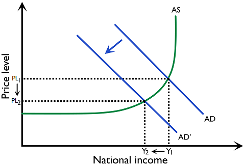
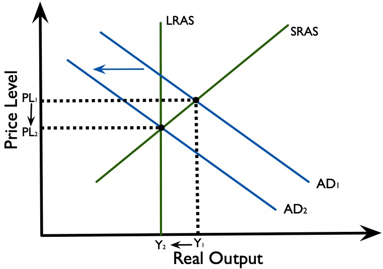
Increasing income tax reduces disposable income, which reduces consumption expenditure and thus AD. Increasing profit tax reduces firms’ retained profits, and reduces investment expenditure and AD. Any of these will lead to a reduction in the AD, and correspondingly, a reduction in price levels and national income (given AS is not vertical), as shown in Figure 3.6.3 and 3.6.4.
The graph below shows that in 2015 Brazil was experiencing high levels of inflation, reaching around 9%. In response, the Brazilian government instituted austerity measures.
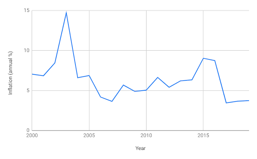
Brazil adopted a constitutional expenditure ceiling in 2016, intended to limit federal primary spending in real terms for twenty years. It linked permitted nominal growth to inflation, with the aim of restraining expenditure relative to GDP. This is a historical policy: a new fiscal framework replaced the ceiling in 2023.
Simulations under the original 2016 framework projected that it would reduce federal expenditure from 19% of GDP in 2017 to 12% of GDP in 2036; the government hoped that this would have a deflationary impact on the economy, and mitigate the effects of the economic crisis.
However, the contractionary policies implemented by the government turned out to be unsuccessful. By 2018, GDP was 5% lower than in 2014, and unemployment had risen from 4.8% to 12.3% over the same time period, leading to increases in the fiscal deficit and public debt despite the austerity measures due to the decline in economic activity and therefore in tax revenue.
Projections under the original ceiling suggested that health and education expenditure would fall from 2.41% of GDP in 2017 to 1.93% in 2026, and that other social and infrastructure spending would fall from around 7% to 2.6%. These were projections under the old rule, not observed outcomes for 2026. Their economic concern remains useful: prolonged restraint on education, health and infrastructure may weaken human capital and productive capacity.
Supply-side effects of demand side policies
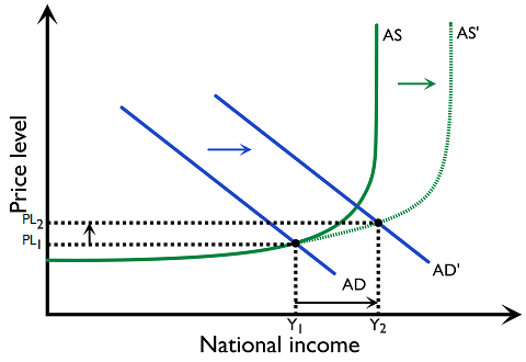
Although fiscal policy is considered as a demand-side policy, it can also have an impact on the supply side. Certain forms of fiscal policy can increase the potential output of the economy, as shown in Figure 3.6.5.
Examples include:
(1) Creating an economic environment friendly to private investment
This includes the reduction of corporate taxes and other forms of incentives that encourage firms to invest. As investment expenditure might increase productivity as well as productive capacity, the AS curve might increase.
(2) Government spending on capital goods
Government provision of roads, for instance, will increase the capital stock of the economy, which can support other forms of economic activity. This would increase the AS in the economy.
(3) Government spending on human capital
This includes increased schooling of young people and training of workers, increasing productive efficiency, and hence increasing the AS in the economy.
The Keynesian multiplier
The nature of the Keynesian multiplier
Multiplier effect means an increase in the initial injection leads to a higher increase in national income (real GDP). Recall the circular income flow model in an open economy; after households receive factor income, they can use it towards four possible uses: (1) Consumption expenditure, (2) Savings, (3) Taxes, and (4) Import expenditure, represented as the outflow of income from households.
For every dollar of income earned by each household, a certain percentage is used in each of the four uses. This percentage is known as the marginal propensity. Marginal propensity to consume (MPC) is the proportion of additional income used for consumption. Marginal propensity to save (MPS) is the proportion of additional income used for savings. Marginal propensity to tax (MPT) is the proportion of additional income paid as tax. Marginal propensity to import (MPM) is the proportion of additional income spent on imports. Because all factors of income go into one of these four uses, their marginal propensities must add up to 1:
MPC + MPS + MPT + MPM = 1
When there is an injection into the system (for instance, through government expenditure), income increases by the amount of the injection at first. However, the increase does not stop there. Assume MPC = 0.5, such that 50% of the additional household income is spent on consumption. With an initial injection of $100, total income increases by $100. The $100 is then paid out to households as factor income by firms. Household income increases by $100. As MPC is 0.5, households spend 50% of their income, which $50 is spent as consumption expenditure on firms. Firms gain $50 and again pay $50 as factor income to households. From the $50 income, households spend $25 on consumption.
The calculation resembles the formula for a sum to infinity of a geometric series. Therefore, the total income generated by this process can be calculated by the following formula:
Total income generated = Initial injection × \( \frac{1}{1-MPC} \)
\( \Delta Y = 100 + 100(0.5) + 100(0.5)^2 + 100(0.5)^3 + 100(0.5)^4 + ... \)
\( = 100 ( \frac{1}{1-0.5} ) \)
\( = 200 \)
The term \( \frac{1}{1-MPC} \) is also known as the Keynesian multiplier; in this case where the initial injection is $100 and MPC=0.5, the multiplier is \( \frac{1}{1-0.5} = 2 \). The total income generated is \( $100 \times \frac{1}{1-0.5} = $200 \). Note that for any multiplier larger than 1, an injection into the economy has a larger effect than the original size of the injection; the same goes for the amount of reduction in national income when leakages from the circular income flow occur. Also, note that there is an alternative formula for the Keynesian multiplier:
Keynesian multiplier: \( \frac{1}{1-MPC} = \frac{1}{MPS+MPT+MPM} \)
where \( MPS + MPT + MPM = 1 – MPC \)
The Keynesian multiplier on AD-AS diagram
To represent the effect of the Keynesian multiplier on the AD-AS diagram, first draw the new AD resulting from an initial injection into the economy, and then the final AD after the multiplier effect takes place, as shown in Figure 3.6.6:
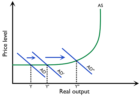
Initially, injections like increased government expenditure by the amount \((Y’ – Y)\) shifts AD from \(AD\) to \(AD’\). Then, the multiplier effect takes place, and the AD is further shifted to the right to \(AD’’\), with \(Y’’\). The new equilibrium real output level has increased by \((Y’’ – Y)\), more than the initial government injection \((Y’ – Y)\). The diagram is only valid when the size of the multiplier is greater than 1.
Effectiveness of fiscal policy
Constraints on fiscal policy
(1) State of economy
The shape of AS plays an important role in determining the effectiveness of the use of fiscal policy. If the economy is at a recessionary gap, the use of fiscal policy would be effective in increasing output. If the economy is near the potential level of national income, an expansionary demand-side policy will not be effective in increasing real output. The effects of fiscal policy on different states of the economy can be summarised as follows: (Figure 3.6.7 and Table 3.6.8)
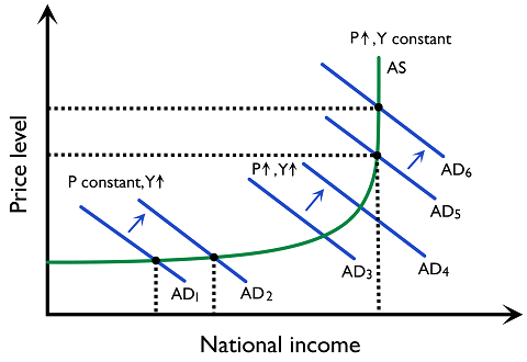
Table 3.6.8: Effectiveness of fiscal policy at different states of the economy
| Shape of AS | State of economy | Price level change | Real output change |
|---|---|---|---|
| Vertical | At physical limit | Large | None/minimal |
| Upward sloping | Below but near physical limit | Moderate | Moderate |
| Flat | Recession | None/minimal | Large |
(2) Crowding-out effect
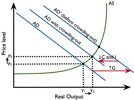
Crowding out is the situation where the government expenditure is higher than the tax revenue, and the government needs to borrow money to finance its expenditure, forcing up interest rates and thereby reducing investment and consumption expenditure. If the government uses an expansionary fiscal policy, it may need to raise debts to finance its spending. Given a pool of funds available for lending, any amount borrowed by the government may reduce the amount available for lending to households and firms, and will drive up interest rates as the supply of loanable funds goes down. The cost of borrowing increases and the investment and consumption expenditures reduce. This reduces the extent of AD increase from an expansionary fiscal policy.
(3) Time lag
There is a time lag between the implementation of a fiscal policy and the effects of real output change to being realised in the market.
(4) Political constraints
Any form of fiscal policy choice will have distributional impacts (e.g. spending programmes targeted at the poor will redistribute wealth from taxpayers to the poor) and may be opposed by those who would lose out. If the political opposition is great, the government may find it difficult to carry through its fiscal policies.
(5) Sustainable debt
In order to implement expansionary fiscal policies, the government may have to run a budget deficit. Over time, this might accumulate into unsustainable national debt.
Strengths of fiscal policy
(1) Targeted
Government expenditure can be targeted at specific areas of the economy. For instance, infrastructure projects can provide jobs to the construction industry, which might suffer badly in the aftermath of a housing bubble.
(2) Direct, and effective during a recession
Government expenditure is a component of aggregate demand and its application will have a direct impact on the AD. Tax cuts directly increase disposable income. This is in contrast to monetary policy, which relies on the banking system lending to provide loans to firms and consumers, which may fail in times of tightened lending or low consumer/business confidence during a recession.
Automatic stabilisers: progressive taxes, unemployment benefits
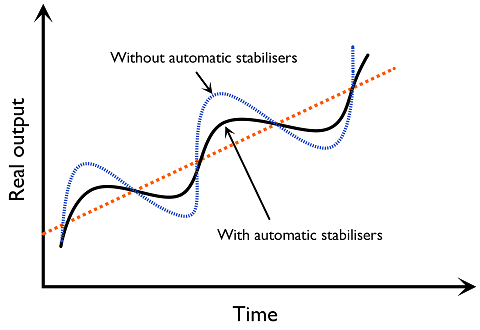
Automatic stabilisers are government tax and expenditure policies that automatically vary with the level of economic activity and national income, and that act to reduce short-term fluctuations in the income level. Income taxes and welfare spending are important automatic stabilisers.
A progressive income tax system is a type of automatic stabiliser. When economic activity increases, household income increases. The proportion of income paid as tax increases. Hence a progressive tax system can slow down the increase in disposable income and AD. When economic activity decreases, household income decreases. The proportion of income paid as tax decreases. Hence a progressive tax system can slow down the decrease in disposable income and AD. A progressive tax system, therefore, can automatically smooth out the fluctuations in the business cycle.
Welfare payment is another type of automatic stabiliser. When national income decreases and the economy experiences a slowdown, unemployment increases. Workers receive unemployment benefit payments, alleviating the fall in their income level and hence AD. When the economy picks up again, benefit claims go down. Welfare payments can therefore automatically smooth out the fluctuations in the business cycle. The effect of automatic stabilisers on the business cycle can be seen in Figure 3.6.10: