3.5 Demand management (demand-side policies) - monetary policy
The central bank, as the government’s banker, plays an important part in the functioning of a country’s financial system. It has various roles, and its specific functions and goals vary according to the country. Central banks are usually responsible for:
- Setting interest rates and/or managing exchange rates
- Regulating and supervising the commercial banks
- Acting as a lender of last resort to commercial banks
In the financial system of one economy, the central bank is the lender to all investment and commercial banks. Investment banks and commercial banks are firms that act as financial intermediaries who bring borrowers and lenders together and aim to maximise profit.
Monetary policy is the control of the supply of money and the interest rate level in the economy by the central bank.
Expansionary monetary policy increases aggregate demand via increasing the money supply and decreasing the interest rate, and contractionary monetary policy reduces aggregate demand via decreasing the money supply and increasing the interest rate.
The goals of monetary policy
The central bank aims to meet the goals of monetary policy, which are:
- A low and stable rate of inflation, usually with ‘inflation targeting’, where the central bank sets a target inflation rate as a goal. The UK’s target inflation rate, for example, is 2%, with a deviation of +/- 1%.
- A low unemployment rate. As the inflation rate and unemployment rate are inversely related, a low and stable inflation rate means that the unemployment rate will also be stable.
- A stable economic environment which helps to achieve long-run growth. Low and stable inflation promotes consumer confidence and encourages investors to invest.
- Reducing fluctuations in the business cycle. Fluctuations occur when the inflation rate changes; by maintaining a low and stable inflation rate, the central bank can avoid such fluctuations.
- Achieving an external balance between export revenue and import expenditure.
The process of money creation by commercial banks (HL)
Commercial banks can create money through ‘credit creation’; that is, they can lend money to customers, individuals and firms, by making loans based on the deposits that customers have made with them. Commercial banks create money by lending out a multiple of the deposit value. This is known as the money multiplier.
Minimum reserve requirement is the percentage of deposits that commercial banks are legally required to hold in reserve so that they can meet customers’ cash requirements, and is set by the government. That is, commercial banks need to maintain a stock of money so that you or I could withdraw some money from an ATM when we want to.
To see how the money multiplier works, imagine that customer A places £100,000 in a bank. Assuming that the bank is required to keep a minimum reserve requirement of 25%, so the bank needs to keep £25,000 as reserves for customer A’s deposit, and the bank has £75,000 of customer A’s deposit that is not being used as reserves. Now suppose that the bank is asked for a loan of £200,000 from business Y, which the bank deems to be credit-worthy and decides to lend out the full £200,000 to business Y. The bank credits business Y’s account with £200,000, while business Y also has a debt of £200,000 in the loan account; by lending to business Y, £200,000 of ‘new’ electronic money has been created and deposited into business Y’s account. Having said that, the bank still needs to meet the minimum reserve requirement of 25% of £200,000, which is £50,000. The bank can do so with the remaining £75,000 from the original deposit. After fulfilling the minimum reserve requirements of £50,000 of business Y’s deposit, the bank still has a remaining of £25,000 from the original deposit, and another £100,000 of new money can be created under the same process if needed.
The money multiplier can be calculated as follows:
If the minimum reserve requirement is 25%:
\[Money\;multiplier=\dfrac{1}{25\%}=4\]
That means that the original deposit of £100,000 can generate £400,000 in new money.
Tools of monetary policy (HL)
Open market operations
Open market operations involve the central bank buying and selling government securities on the open market. Government securities are bonds that offer interest on their nominal rate which are redeemable after a given number of years. They are considered to be very low-risk because they are guaranteed by the government.
The central bank can reduce the money supply by selling more bonds to institutions; this reduces the money that commercial banks have available to lend. This will increase the cost of borrowing and therefore increase interest rates. Higher interest rates lower AD as they discourage spending and investment and encourage saving. This is a contractionary monetary policy.
The central bank can also increase the money supply by buying back bonds from institutions; this increases the money that commercial banks have to lend, driving down the cost of borrowing and interest rates. This shall increase consumption and investment expenditure. As C and I are components of the AD, this will increase AD.
Minimum reserve requirements
Minimum reserve requirement is the percentage of deposits that commercial banks are legally required to hold in reserve so that they can meet customers’ cash requirements, and is set by the government. The larger the minimum reserve requirement, the lower the multiple of deposit value that can be created from the initial deposits, the smaller the money multiplier. The government can therefore reduce the money supply by increasing the minimum reserve requirement, thus reducing banks’ ability to create credit. If the government wants to increase the money supply, it can reduce the minimum reserve requirement; this increases the ability of banks to create credit. Increased amounts of credit incentivise consumer spending and investment by firms; this shifts out AD, leading to economic growth.
Changes in the central bank minimum lending rate
The minimum lending rate, or base rate, is the rate of interest which the central bank charges on loans and advances to commercial banks. It therefore influences the interest rate elsewhere in the economy, such as on bank loans and mortgages.
The central bank can implement a contractionary monetary policy by raising the minimum lending rate; this will push commercial banks to raise their lending rates and their interest rates, and thus encourage consumers and businesses to reduce their consumption and increase their savings. This will reduce AD.
The central bank can implement an expansionary monetary policy by lowering the minimum lending rate; this will push commercial banks to lower their lending and interest rates, encouraging consumers and businesses to save less and spend more. This will increase AD.
Quantitative Easing
Quantitative easing is an expansionary monetary policy that involves the central bank introducing new money into the economy through the purchase of assets from commercial banks and other financial institutions e.g. corporate securities, mortgage backed securities etc.
QE can help to increase AD because:
- As the commercial banks sell off securities, the commercial banks’ reserves as well as its liquidity increase, encouraging the commercial banks to lend more to consumers and investors, and thereby encouraging consumption and investment expenditure, and AD.
- QE also helps to lower the interest rate, and therefore reduces consumers’ and firms’ interest repayment when they take out a debt; this should increase both the consumer and business confidence, hence increasing consumption and investment expenditure, and AD.
- Lower interest rates will lead to the exchange rate falling, making exports less expensive and imports more expensive. This will increase net exports and therefore AD.
Determination of equilibrium interest rates
Interest rate refers to the price of borrowing. The interest rate is determined by money demand and supply in the market.
Money demand
Money plays an important part in the functioning of an economy. People demand money (in the form of cash) for various uses:
(1) Transactional demand
Money can be used as a medium of exchange when purchasing goods and services. With a greater consumption level due to an increase in income, wealth or price, the demand for money increases.
(2) Precautionary demand
Money is held for emergency purchases, such as emergency medical bills. Inventions that make access to money easier, such as automatic teller machines (ATMs), decrease precautionary demand.
(3) Speculative demand
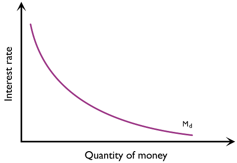
Money, as stored value, can be held by speculators in the hope that its real value may increase in the future. Holding money incurs opportunity cost of foregoing the interest rate earned. When money is held, the interest rate is given up. The interest rate can be understood as the price of holding money. The lower the interest rate, the lower the cost of holding money. Therefore the demand curve for money is downward sloping, as shown in Figure 3.5.1.
Money supply
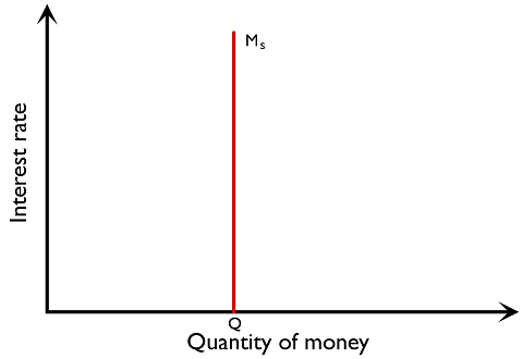
There is also a supply side to the money market, and that is determined by the central bank. The central bank controls the monetary base in the economy e.g. printing cash. The monetary base, together with deposit created by commercial banks, forms the economy’s money supply.
Assume that the central bank can set the money supply at any quantity independent of the level of the interest rate. The supply curve for money is vertical (as seen in Figure 3.5.2).
Determination of equilibrium interest rates
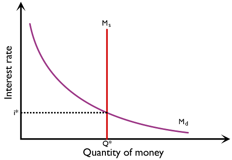
The equilibrium of money demand and supply determines the interest rate, as seen in Figure 3.5.3. Since the central bank can control the level of money supply in the economy, it can influence the equilibrium level of interest rates in the economy, subject to the level of money demand.
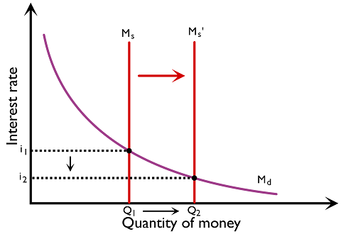
If the central bank increases the money supply, there is more money available in the market, which lowers its price and thus decreases the interest rate.
If, on the other hand, the central bank decreases the supply of money, there is less money available in the market and will bid up its price, increasing the interest rate.
Real versus nominal interest rates
The nominal interest rate is the interest rate available in the money market, not adjusted for inflation. The real interest rate is adjusted for inflation.
The real interest rate = the nominal interest rate - the inflation rate
The nominal interest rate is 6%. The inflation rate is 2%. Calculate the real interest rate.
Real interest rate = nominal interest rate - inflation rate
Real interest rate = 6% - 2%=4%
The real interest rate is important for the real gain analysis. If the nominal interest rate is 6%, while inflation rate is 2%, the real interest rate, representing the real gain from investment would only be 4%. This is particularly significant when the interest rate becomes negative, as anyone saving will find that the value of their savings is actually decreasing over time.
Expansionary and contractionary monetary policies to close deflationary/recessionary and inflationary gaps
Monetary policy is a demand-side policy using changes in the money supply or interest rates to affect AD to achieve economic objectives relating to inflation and unemployment.
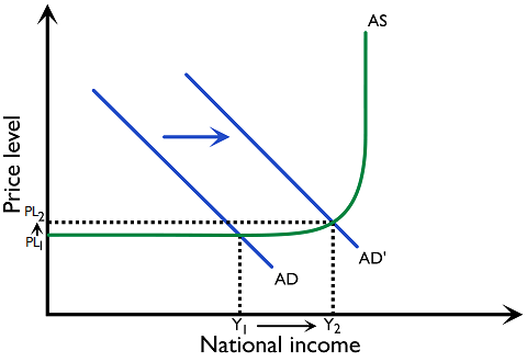
Expansionary monetary policy means reducing interest rates by increasing money supply (see Figure 3.5.4) to increase aggregate demand. A lower interest rate reduces the cost of borrowing, which encourages households and firms to take up new loans to consume and invest. As consumption and investment expenditure increase, aggregate demand increases from AD to AD' (see Figure 3.5.5). The effects on price level and national income will depend on the shape of the AS curve.
The 2008 financial crisis was a worldwide financial crisis caused by excessive risk-taking by banks and a downturn in the subprime lending market in the United States, which led to the bankruptcy of the bank Lehman Brothers. The 2008 financial crisis led to the Great Recession, and was followed by the European debt crisis.
The 2008 financial crisis led to a contraction in US real GDP: the April 2009 BEA advance release reported annualised falls of 6.3% in the fourth quarter of 2008 and 6.1% in the first quarter of 2009. These figures were subsequently revised. An annualised fall of 6% is equivalent to about 1.53% within one quarter. The crisis also led to the US unemployment rate rising to 10.1% by October 2009. The PEW Research Centre found that, on average, US households lost nearly $5,800 in income due to the reduced economic growth during the crisis, with the US losing $3.4 trillion in real estate wealth from July 2008 to March 2009 and $7.4 trillion in stock wealth from July 2008 to March 2009.
The Federal Reserve (commonly known as ‘the Fed’) is America’s central bank. The chair of the Federal Reserve during the financial crisis was Ben Bernanke; there is also a vice chair, and five other members of the Federal Reserve Board of Governors. Alongside the Board of Governors, there are twelve regional banks, which are responsible for particular geographic regions.
Unemployment in the US had been rising even before the financial crisis. The Fed therefore began reducing interest rates in September 2007, and reduced them steadily until June 2008. The graph below shows the US discount-rate series between 1950 and 2019, rather than the federal-funds target rate, and illustrates the steep drop in the interest rate in response to the financial crisis.
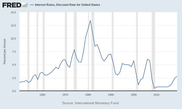
With the federal-funds target range reduced to 0–0.25% in December 2008, the Fed began to use ‘unconventional’ monetary policy.
In August 2007, the Fed announced that interest rate cuts might be coming; this was ‘forward guidance’, which was intended to influence individuals’ and firms’ perception of what the interest rate was going to be in the future, and therefore to alter households’ and firms’ financial decisions to boost the economy.
Another ‘unconventional’ monetary policy carried out by the Fed was quantitative easing. This was carried out in several stages:
- QE1 began in November 2008, when the Federal Reserve announced purchases of up to $100 billion of agency debt and $500 billion of agency mortgage-backed securities (MBS). In March 2009, it announced an additional $750 billion of MBS purchases, bringing the planned MBS total to $1.25 trillion, and an additional $100 billion of agency debt purchases. It also announced purchases of up to $300 billion of longer-term Treasury securities.
- QE2 began in November 2010, when the Fed bought $600 billion worth of longer-dated treasury bonds between November 2010 and mid 2011.
- Operation Twist began in September 2011, and involved the Fed buying $400 billion worth of longer-dated treasury bonds and selling off the same amount of shorter-dated bonds.
- QE3 began in September 2012, with the Fed committing to buying $40 billion of mortgage-backed securities per month. This began to taper off in December 2013, and ended in October 2014.
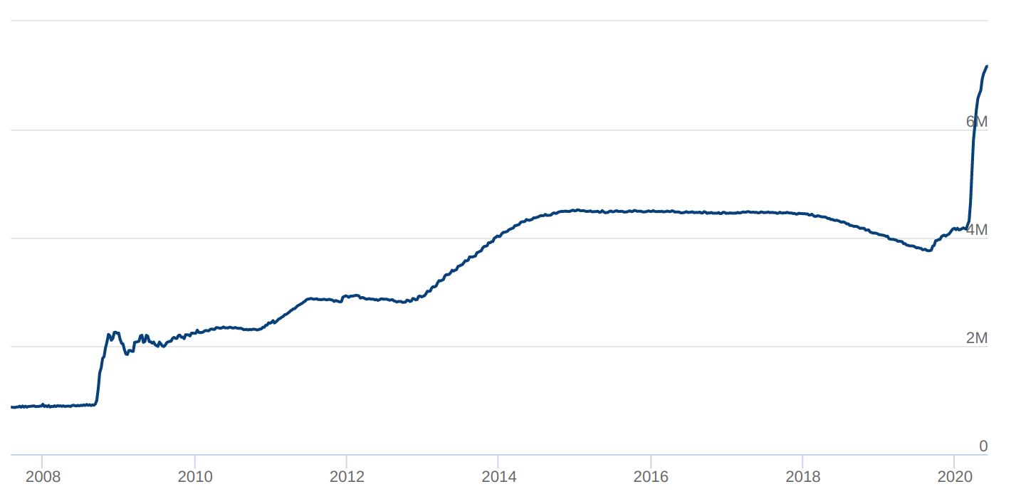
The graph below shows the Fed’s balance sheet from 2007 to 2020. It shows that the total assets owned by the Fed increased from $870 billion in August 2007 to $4.5 trillion in early 2015, reflecting the impact of quantitative easing.
However, not all of the money that was created by the Fed actually made it into circulation. Many banks stockpiled excess reserves, as shown by the graph below.
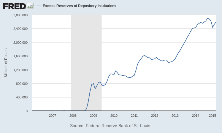
Overall, QE in the US seems to have been successful in dealing with the financial crisis; both economic growth and the unemployment rate improved significantly since 2008. For example, Ben Bernanke claimed that QE1 and QE2 increased economic activity by 3% and added 2 million jobs to the economy. However, most studies agree that QE1 was the most effective round, and that the later rounds had less of a positive effect on the economy. It is also argued that the excess reserves held by banks after the financial crisis might lead to higher inflation in the future. Savers have also lost out from QE, with some estimates saying that QE has cost savers around $360 billion.
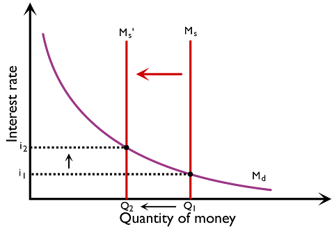
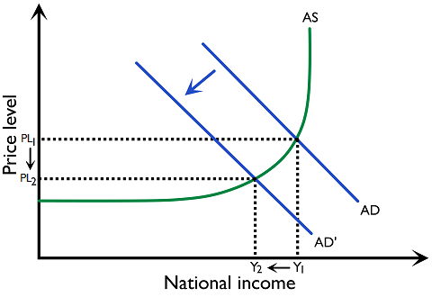
Conversely, contractionary monetary policy means the central bank reduces money supply (see Figure 3.5.6) in the economy to increase the interest rate and hence decreases aggregate demand. Increasing the interest rate increases the cost of borrowing and reduces the level of consumption and investment expenditure. Aggregate demand decreases from AD to AD' (see Figure 3.5.7). The effects on price levels and national income will depend on the shape of the AS curve.
The annual inflation graph below illustrates the high inflation of the 1970s. Monthly year-on-year CPI-U figures are a different measure: BLS index levels imply inflation of approximately 9.4% in January 1974 and 12.3% in December 1974. These monthly observations should not be read directly from the annual graph.
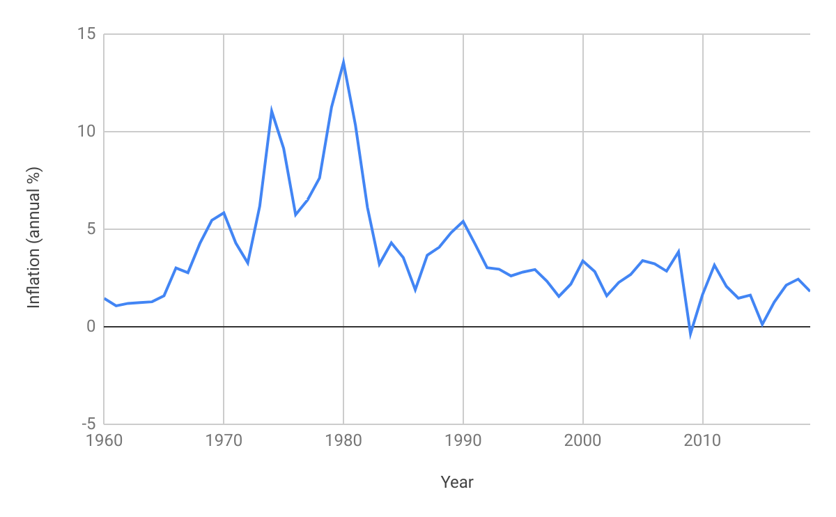
In response, the Fed raised interest rates to almost 13% in July 1974. However, this failed to reduce inflation, and economic growth was slow despite the high rate of inflation; this combination of slow economic growth and high rates of inflation is known as ‘stagflation’. There was strong political pressure for the Fed to reduce interest rates again, which it did in 1975, where interest rates dropped to 7.5%.
In 1979, Paul Volcker became the chair of the Fed. He oversaw an increase in the interest rate to a peak of 20% in 1981; this finally led to a decrease in inflation, which dropped back to pre-1970 levels by the mid 1980s.
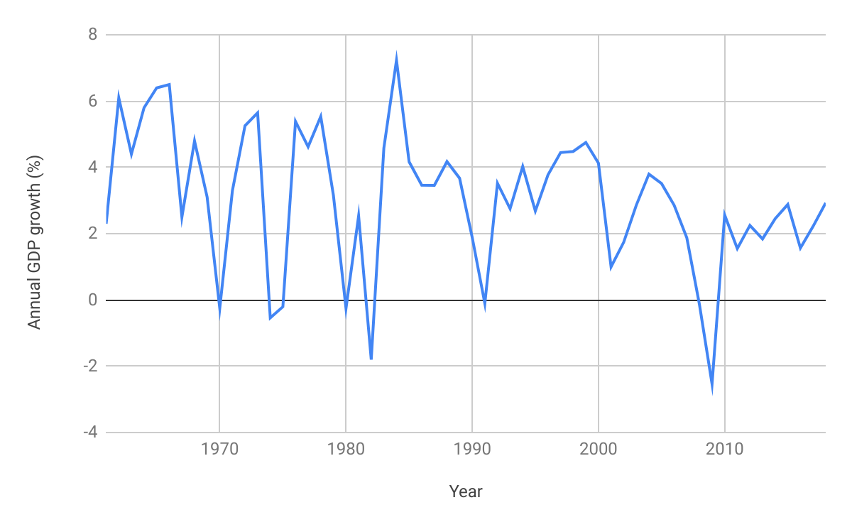
However, this aggressive contractionary monetary policy severely weakened the US economy, and contributed to two recessions in the early 1980s. The graph below shows annual GDP growth in the US between 1960 and 2019, and illustrates the steep economic downturn in the early 1980s.
Effectiveness of monetary policy
Strengths of monetary policy
(1) Ability to implement changes in rates quickly
Central banks are able to vary money supply and interest rates promptly, thus are able to respond to changes in macroeconomic conditions quickly, granting it a degree of flexibility that fiscal policy cannot match.
(2) Ability to adjust rates incrementally
Central banks are able to adjust the interest rates 0.25% at a time, and therefore suited to fine-tuning the economy through gradual and incremental changes.
(3) No budget burden
Unlike the expansionary fiscal policy, an expansionary monetary policy does not place a burden on government finances.
(4) Independent central bank is less susceptible to political pressure
If the central bank operates independently from the government, it is able to achieve macroeconomic objectives without political pressure or interference.
(5) Absence of ‘crowding out’
Expansionary fiscal policy which involves increased government borrowing might lead to higher interest rates and ‘crowding out’ of private investment; this is not the case with monetary policy.
Weaknesses of monetary policy
(1) Ineffectiveness during recession
In periods of deep recession, consumer and investor confidence is low. Consumption and investment expenditure are less responsive to interest rate change. This is known as being 'interest inelastic'. Furthermore, during a recession interest rates might already be low because the central bank has already used expansionary monetary policy. This makes future uses of expansionary monetary policy harder.
(2) Time lags
There is a time lag between implementation of monetary policy and full effects to be seen, making monetary policy less effective at the beginning of implementation.
(3) Conflict among government economic objectives
Use of monetary policy might help attain one of the macro-objectives, but at the same time it will trade off other objectives. For example, the use of an expansionary monetary policy can increase real output level, yet this might incur a higher inflation level.
It is important to evaluate the effectiveness of monetary policy by considering the shape of the AS curve.
If the AD is originally at the horizontal or mildly upward sloping portion of the AS curve, the shift in AD caused by an expansionary monetary policy is effective in influencing the level of real output.