3.3 Macroeconomic objectives
Economic growth
One of the goals of macroeconomic policy is to promote economic growth. Economic growth is the increase in real output in an economy over a period of time.
Short-term growth/ Actual economic growth
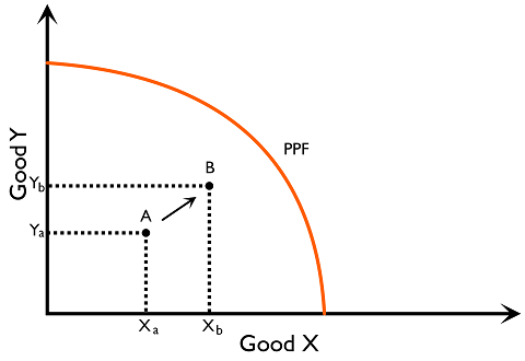
There may be inefficiencies with the way that existing resources in the economy are used. On the PPF, this can be represented by the points inside the production possibilities frontier. The further away the actual production point is from the frontier, the more inefficiency there is.
Actual economic growth is the increase in real GDP in the economy through making better use of unused resources with no change in the stock of productive resources. Without changes to the quantity and quality of existing resources, the actual production point can be moved closer to the frontier by better utilising resources, or in the reduction of unemployment.
This can be shown in the PPF diagram of an economy producing good X and Y in Figure 3.3.1. When there is an increase in actual output from point A to B, the economy is producing more of both goods (compare the bundles \((X_a, Y_a)\) and \((X_b, Y_b)\)) without a change to the productive capacity of the economy. Point B is also closer to the frontier than A.
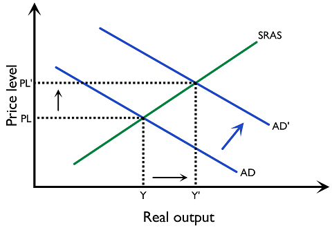
This can also be illustrated using an AD/AS diagram. An increase in aggregate demand from AD to AD’ leads to an increase in real output from Y to Y’. As there has been an increase in real output, so there has been an increase in real GDP and therefore economic growth.
Long-term growth/Potential economic growth
Potential economic growth is the increase in potential productive capacity in an economy.
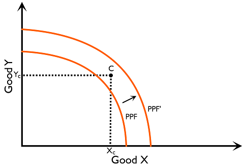
When there are improvements in quality and availability of any factor of production (labour, capital, land and entrepreneurship), the level of output that can be produced in the economy increases. This can be shown in the PPF in Figure 3.3.3. As the PPF shifts to the right, combinations with larger quantities of goods are made available. Combination C of good X and Y that was not feasible under the previous PPF now becomes feasible under the expanded production possibilities at PPF’.
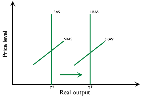
The above change in production possibilities can also be shown by the rightward shift of the aggregate supply curve from LRAS1 to LRAS2 in Figure 3.3.4, which indicates the level of potential output of the economy increases from Y* to Y*'.
Measurement of economic growth
We can calculate the rate of growth using the following formula:
\( Growth\;rate=\dfrac{Real \; GDP \; in \; year \; 2 \; - \; Real \; GDP \; in \; year \; 1}{Real \; GDP \; in \; year \; 1} \times 100 \% \)
In 2009, the real GDP of the US was USD $12,880.6 billion. In 2010, the real GDP had changed to USD $13,248.7 billion. What is the rate of economic growth between 2009 to 2010?
\( = \dfrac{13,248.7 - 12,880.6}{12,880.6} \times 100\% \)
\( = 2.86 \% \)
Consequences of economic growth
(1) Living standards
Higher economic growth leads to more job opportunities and a higher level of income. With a higher income level, people’s living standard increases. For example, people can afford to dine out, move to a bigger place etc.
(2) Unemployment (or employment)
Economic growth can bring different effects to different members of the labour force. On one hand, an increase in economic activity through growth is associated with the creation of new employment opportunities and has a positive effect on employment in the economy. On the other hand, economic growth is often associated with changing production patterns. An example of this would be automated production, which favours labour with know-how in operating machinery and disfavours labour with manual skills. Workers who find their skills no longer demanded by the economy might find themselves structurally unemployed (or technologically unemployed).
(3) Inflation/deflation
Higher levels of economic activity induce a higher demand for scarce productive resources, which may push up factor prices, and consequently, the general price level in the economy. Yet, increased productivity and technology shifts the aggregate supply curve towards the right, and induces a downward trend in prices when economic growth results from increased productivity.
(4) Distribution of income
The returns to economic growth need not be distributed evenly. If economic growth causes a relatively higher increase in income level for the rich than the poor, then the income gap widens and income inequality increases. However, if the harvest from economic growth can be distributed evenly across all levels of society, then income distribution can be improved.
(5) The current account of the balance of payments
As economic growth can possibly lead to a higher price level in an economy, the domestic export price level increases. This reduces the competitiveness of domestic exports and reduces export revenue. Concurrently, imported goods become relatively cheaper compared with domestic products. The level of import quantity might increase, thus increasing import expenditure in the economy. As a large portion of the current account is measured by export revenue minus import expenditure, the current account balance might worsen.
(6) Impact on the environment
Economic activity and growth also make use of natural capital provided by the environment. High rates of economic growth may not be sustainable if it leads to the depletion of natural resources. For instance, when the green GDP measure was adopted in China in 2004 to assess the environmental impact brought by economic activities, certain provinces had growth rates close to zero when the costs of environmental damage were taken into account. This echoes with the point about living standards. Economic growth might have an adverse impact on the standard of living if environmental costs of growth are huge.
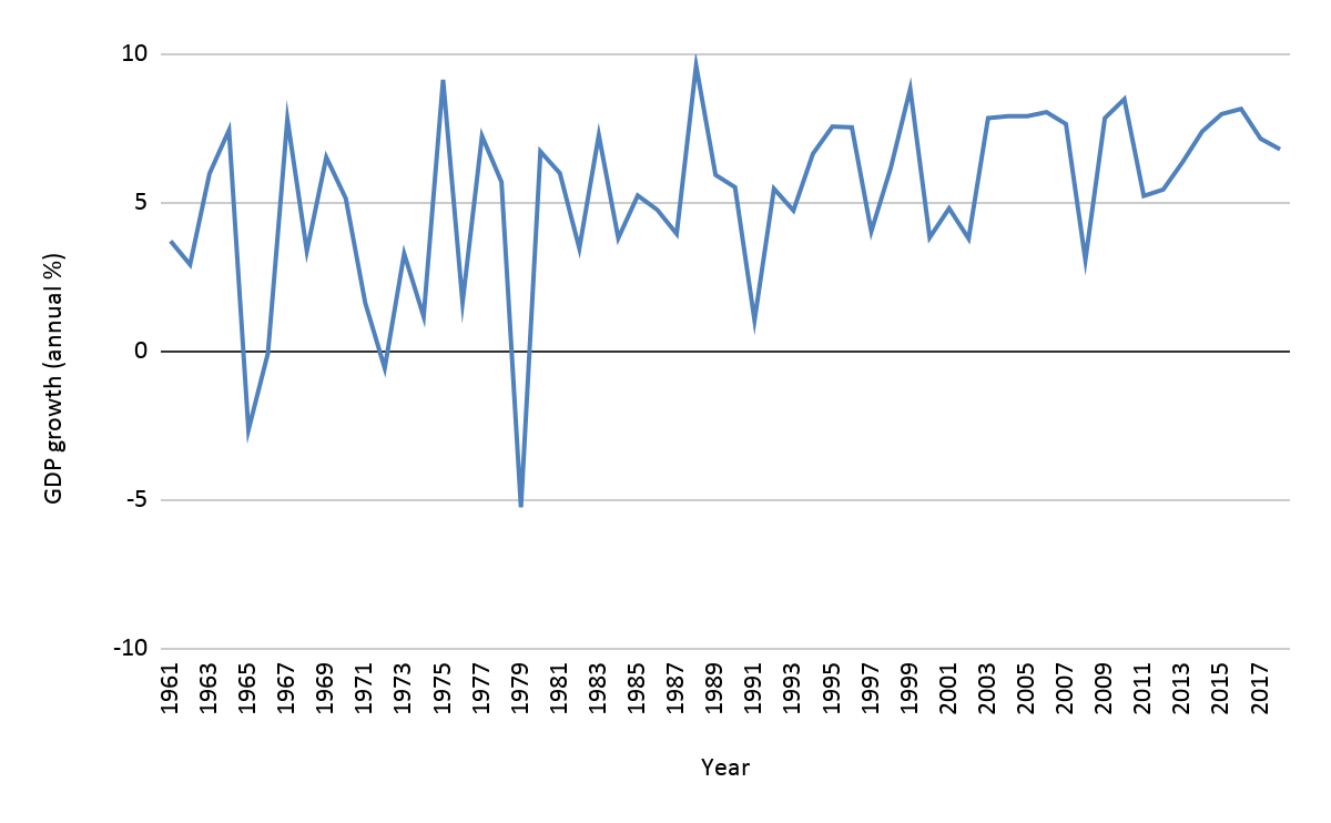
To analyse the consequences of economic growth, consider the example of India; India is one of the BRIC economies, meaning that it is on its way to becoming a developed country. From 2014 to 2018, India was the world’s fastest-growing major economy.
The graph below shows India’s annual percentage GDP growth from 1961 to 2018. It shows that India’s economic growth has averaged around 6-7% for the last several years.
To some degree, this high level of economic growth has been associated with rising living standards. For example, the graph below shows the percentage of the population living in absolute poverty in India. Although there are only a few data points available, the data clearly shows a downward trend in India’s absolute poverty rate over time.
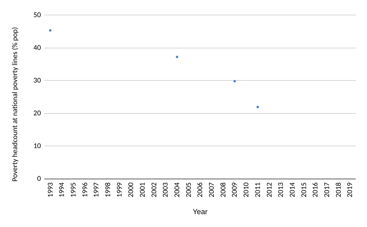
However, India’s poverty rate is still very high; between 20 and 30% of its population are living in absolute poverty.
Data context: The 20–30% estimate above is retained from the original case. Its survey date and poverty-line definition are not specified, so it is not a verified current estimate and should not be directly compared with a differently defined rate. The World Bank updated its international extreme-poverty line to $3.00 a person per day in 2021 PPP prices in June 2025. Earlier $1.90 figures use 2011 PPP prices. PPP dollars are purchasing-power-adjusted units, not amounts converted at market exchange rates. Old poverty percentages cannot be relabelled with the new threshold; they require recalculation from the underlying survey data. World Bank: June 2025 update
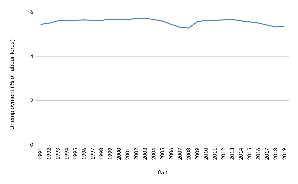
The graph below shows India’s unemployment levels between 1991 and 2018. It indicates that persistently high levels of economic growth have given India a low level of unemployment of between 5 and 6% of the total labour force since 1991. However, given the size of the informal sector in India, this figure may not accurately represent the true unemployment rate in the country. It also does not reflect underemployment, which has been a significant problem in the Indian economy.
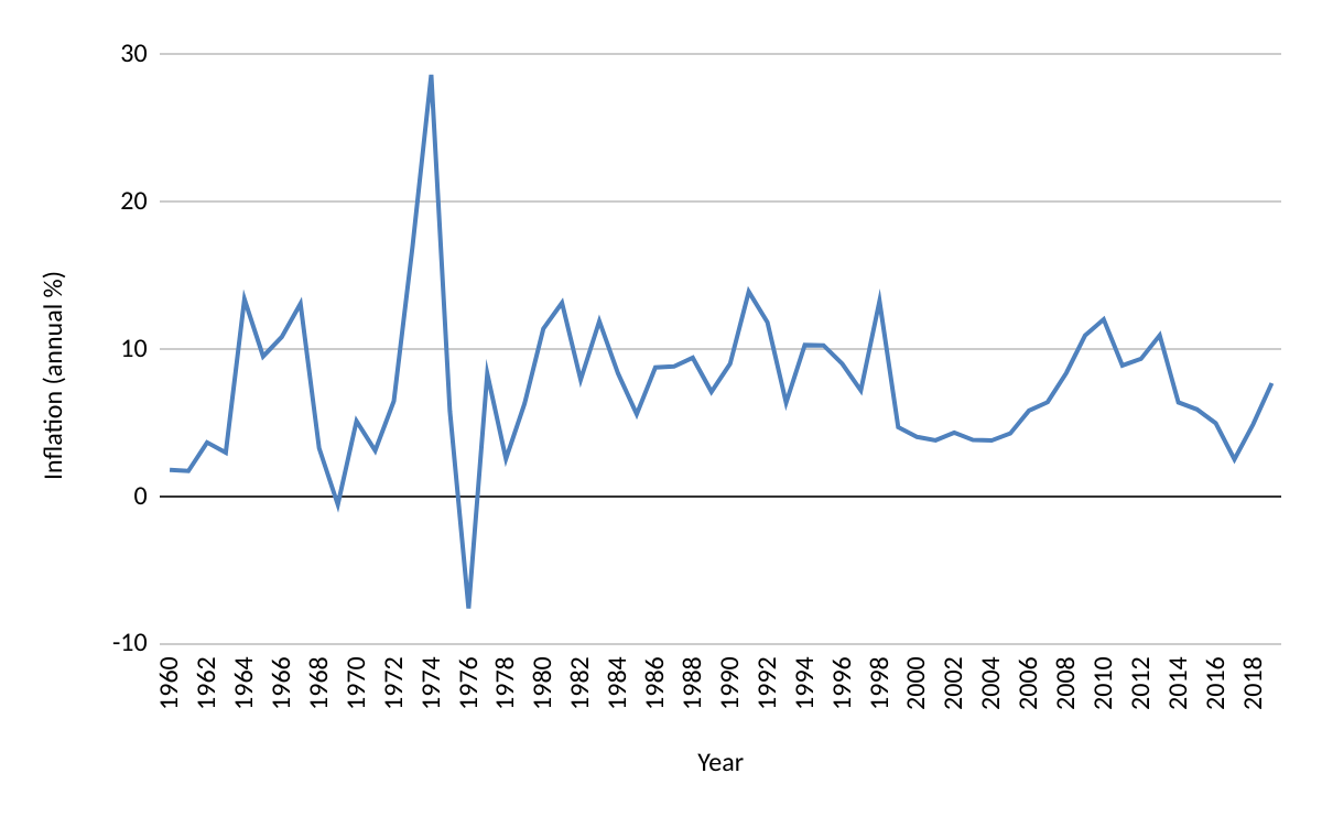
The graph below shows India’s annual inflation rate from 1960 to 2018. It indicates that although India has enjoyed a strong rate of economic growth, this has been accompanied by high inflation; since 1960, India’s inflation rate has averaged around 5%.
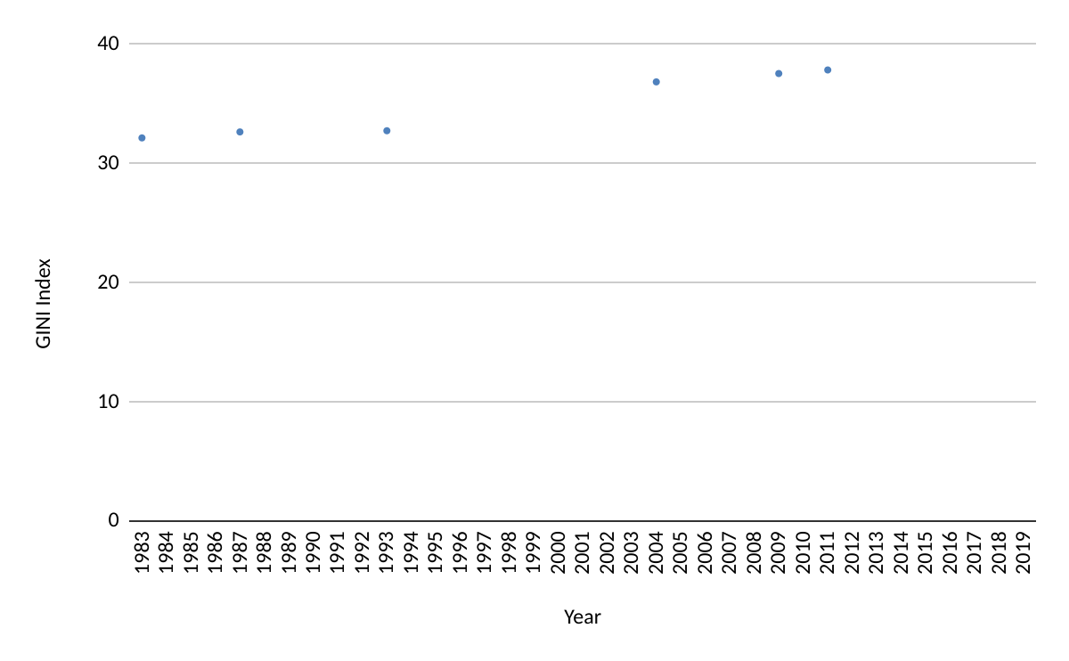
India’s economic growth has also not necessarily led to a more equal distribution of income over time. The graph below shows India’s Gini Index; India’s high Gini coefficient suggests that it has a high level of income inequality, and the graph indicates that this has been rising over time. The benefits of economic growth are therefore not equally distributed among all Indian citizens.
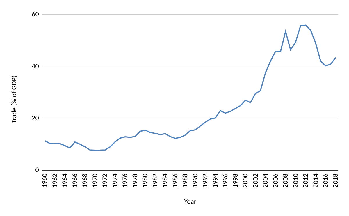
As can be seen from the graph below, trade makes up a significant proportion of India’s GDP. This proportion has been rising along with India’s economic growth, suggesting that India has been able to take advantage of its comparative advantage to achieve export-led growth.
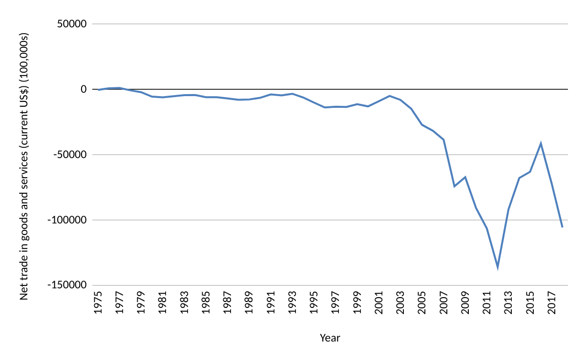
India runs a persistent trade deficit. The graph below shows its net trade in goods and services:
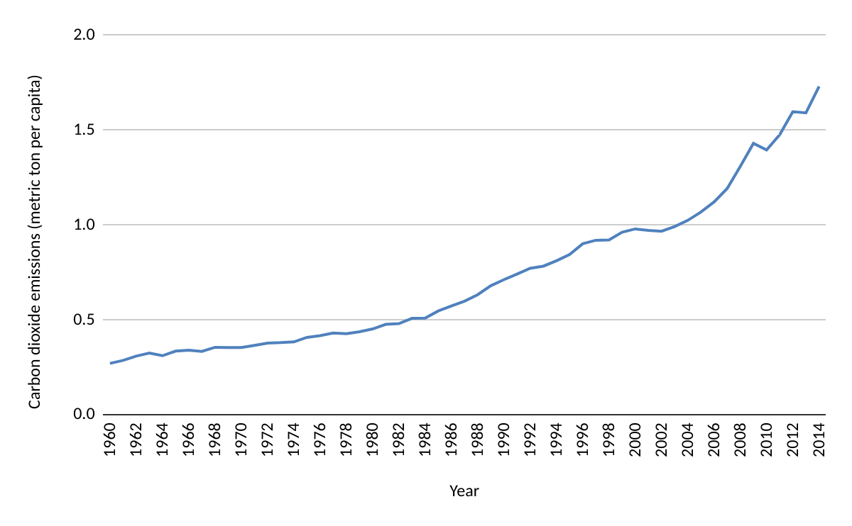
India’s high levels of economic growth have also caused damage to the environment. The graph below shows India’s level of per capita CO2 emissions; as India has experienced high levels of economic growth, its per capita emissions have also increased significantly.
Overall, although India has experienced high levels of economic growth, leading to a rapid increase in per capita incomes, it still has a significant proportion of people living below the poverty line, low per capita incomes, poor life expectancy and literacy rates, and high inflation. India’s future growth is limited by poor infrastructure and human capital, as well as its high inflation rate and low national savings as a share of GDP.
Therefore, while India has enjoyed impressive levels of economic growth, its economic development has been limited by structural problems, which will have to be overcome for it to be able to enjoy similarly high levels of growth in future.
Low unemployment
Unemployment refers to the number of individuals in the labour force that are without work, and willing and able to work, as well as actively seeking for a job.
Measuring unemployment
Unemployment can be expressed as the total number of unemployed individuals in the economy. It can also be expressed as a percentage, calculated by:
\( Unemployment \; rate = \dfrac{Number \; of \; unemployed}{Total \; labour \; force} \times 100 \% \)
Note that unemployment does not refer to any person in the population who does not have a job. The following conditions need to be satisfied:
- The person needs to be in the labour force: this excludes children, students, retirees, people who cannot work due to illness, and people who do not want to be in the labour market (e.g. housewives).
- The person needs to be actively looking for a job: By looking for a job, a person indicates his/her interest in participating in the labour market.
Using the data below, calculate the UK’s unemployment rate in March 2020.
| Number of people unemployed | Size of the labour force |
|---|---|
| 1,348,000 | 33,810,000 |
Unemployment rate \(=\dfrac{1,348,000}{33,810,000}\times 100\%=3.99\%\)
Difficulties in measuring unemployment
Unemployment statistics may not reflect the true extent of unemployment due to the following factors:
(1) Hidden unemployment
Individuals may give up looking for a job when they cannot find employment after a long time period. Known as discouraged workers, these individuals might be willing to work should there be an opportunity. However, official unemployment statistics do not count discouraged workers, and thus tend to understate unemployment.
(2) Underemployment
Underemployment refers to employment that does not make full use of worker capacity. One type of underemployment is involuntary part-time work, where workers who want to and are able to work full time can only find part-time work. e.g. Ski instructors work mostly in winter.
(3) Unemployment rate is a measure of averages
Unemployment rate is an average measure and ignores possible discrepancies in unemployment between regions, ethnic groups, age groups, or genders. For example, there are large differences in the unemployment rates between western and eastern Germany, which are not reflected in nation-wide statistics.
Types and causes of unemployment
When an economy is at ‘full employment’, unemployed workers still exist, and they make up what is known as the natural rate of unemployment. The natural rate of unemployment refers to any unemployment present when an economy is producing at its potential level of output. At its natural rate, an economy is said to be at ‘full employment’ level of output. It includes frictional, structural, and seasonal unemployment.
(1) Frictional unemployment
Frictional unemployment is also called search unemployment. Workers have different skillsets and are a better match for certain jobs. Workers may not find the right jobs straight away due to information costs and would, therefore, spend time searching for the right jobs.
(2) Structural unemployment
Structural unemployment is long-term unemployment that is caused as a result of a decline in the demand for a particular type of labour. Unemployment occurs because there is a mismatch between the skills of unemployed workers and the jobs available. These mismatches are caused by:
i) Changes in demand for particular labour skills
Technological changes and automation which reduce the number of workers required. Workers are said to be structurally unemployed, as they cannot easily find jobs with obsolete skill sets.
ii) Changes in the geographical location of industries
Structural unemployment can also be caused by mismatches in geographical locations. In this case, there are jobs for workers with the right skill requirements but workers would need to relocate. When the costs associated with relocation are too great (such as the costs of learning a new language), workers do not take up these jobs.
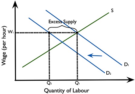
Figure 3.3.5 shows the impact of a fall in the demand for manufacturing labour in a particular area. Assume that the labour wage is at W1. When demand for labour decreases from D1 to D2, and the supply of workers stays the same, at \(W_1\), there is an excess supply of labour between \(Q_2\) and \(Q_1\).
iii) Labour market rigidities
Rigidities in the labour market can also cause structural unemployment. Policies intended to improve labour welfare, such as the minimum wage legislation, may increase the cost of hiring labour to the extent that employers turn to automation as an alternative means of production.
(3) Seasonal unemployment
Seasonal unemployment occurs because the demand for labour in certain industries is higher in certain periods of the year and lower in other periods, e.g. construction and tourism industries. During the off-season when the labour demand is low, workers may find themselves temporarily out of work until the next peak season. Due to the industry’s nature, seasonal unemployment always exists e.g. Ski instructors work more in winter.
(4) Demand-deficient/Cyclical unemployment
Demand-deficient unemployment is caused by insufficient aggregate demand such that the equilibrium level of real output (in the short run) is at a level below an economy’s potential real output level. Aggregate demand, driven by expectations, can remain at low levels when poor business and consumer confidence hinders investment and consumption.
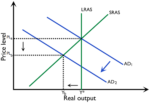
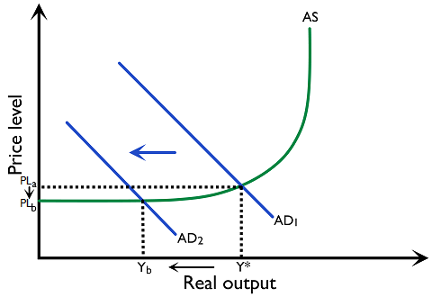
Demand-deficit unemployment can be shown in an AS-AD diagram by shifting the AD to the left from \(AD_1\) to \(AD_2\), which leads to a deflationary gap as \(Y_b\) is lower than \(Y^*\), which is the full employment level of output (Figure 3.3.7 and Figure 3.3.8). When the economy is at \(Y_b\) there is demand-deficient unemployment.
Costs of unemployment
Personal costs
(1) Loss of income
People who are unemployed will receive less income than they would if they were employed, assuming that they are able to receive some unemployment benefits. This will reduce their standards of living and the standards of living of their families.
In the UK in 2020/21, the Universal Credit standard allowance for an eligible single claimant aged 25 or over was £409.89 a month, including the temporary pandemic uplift. Universal Credit is means-tested, and entitlement depends on household circumstances. This is a historical allowance, not the current rate. This may mitigate the loss of income associated with unemployment, but is a small amount in comparison to many wages; for example, it is estimated that average monthly costs while living in London are around £824.72, without accounting for rent costs.
(2) Mental health
A person who remains unemployed over a long period of time could suffer issues with their mental health, as they might suffer from high levels of stress, anxiety, and depression.
The Canadian Institute for Work and Health produced a report in 2009 which analysed the impact of unemployment on mental health. They found significant evidence that becoming unemployed has a negative impact on mental health; for example, a 1999 review paper by Murphy and Athanasou which reviewed 16 studies on the effects on mental health found that 14 of those 16 studies showed a significant negative association between unemployment and mental health.
The report cites several ways in which unemployment can lead to worse mental health: lower standards of living caused by unemployment might affect mental health; insecurity of income might lead to anxiety about the future; unemployment can be associated with stigma and a loss of self-esteem, and losing one’s job may also mean losing the social contacts associated with work, leading to a shrinking of social networks.
Economic costs
(1) Loss of real GDP
With unemployed workers, the economy is producing at a lower output level. The economy is not fully utilising its productive resources and is producing inside its production possibilities frontier (PPF). Unemployment, especially over a prolonged period, also leads to a deterioration and loss of productive skills which also leads to a loss in real GDP.
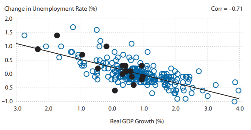
Okun’s Law is derived from the empirical relationship between unemployment and production. It states that when unemployment increases, production is likely to decrease.
A particular rule-of-thumb form of the law is that a 1% increase in the unemployment rate will be associated with a 2% drop in inflation-adjusted GDP growth. The empirical backing of the law is very historically stable, particularly in the United States; this means that many economists in the US have used the law to make macroeconomic predictions and policy proposals.
The graph below compares changes in real GDP growth and change in the unemployment rate in the United States, with the black circles indicating measurements taken during and after the Great Recession. It indicates a strong correlation between the unemployment rate and the growth rate of GDP.
https://files.stlouisfed.org/files/htdocs/publications/review/12/09/399-418Owyang_rev.pdf
(2) Loss of tax revenue
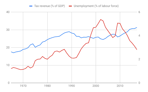
As unemployed workers do not earn a work income, the government takes in less tax revenue.
The graph below compares the unemployment rate as a percentage of the total labour force and tax revenue as a proportion of GDP in Japan between 1965 and 2017. It shows that in times of relatively higher unemployment, such as between 1995 and 2010, tax revenue tends to be below the long-term trend, and in times of low unemployment tax revenue tends to be higher.
(3) Cost of unemployment benefits
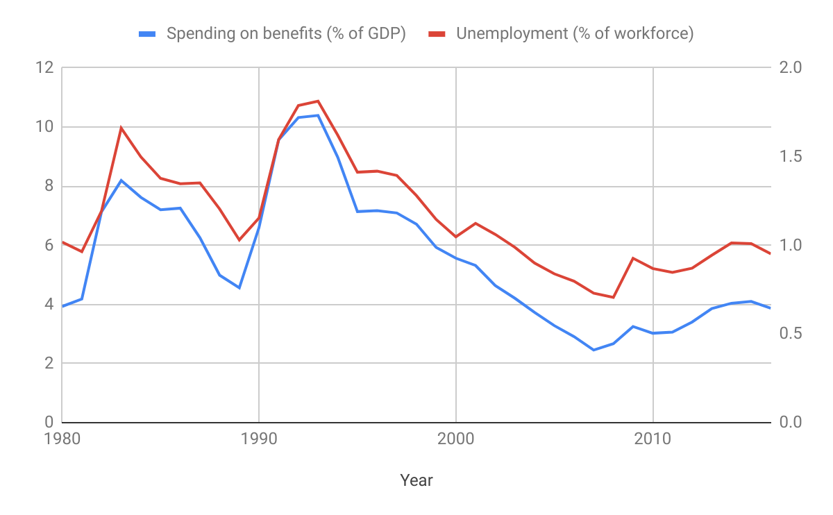
If the government provides unemployment benefits, some of the financial resources that could have been used for the provision of public or merit goods are not used for these purposes. High levels of unemployment may put pressure on a government’s fiscal conditions.
The graph below shows Australia’s spending on benefits as a percentage of GDP alongside its unemployment levels as a percentage of the workforce between 1980 and 2016. It clearly shows that there is a strong correlation between the level of unemployment in the economy and the amount that the government spends on unemployment benefits.
This increased spending on unemployment benefits means that the government has less budget to spend on other public services, such as education and healthcare.
(4) Greater disparity in the distribution of income
There exists a disparity in the distribution of income between those who are working and those who are not. The income and wealth gap between individuals who experience long-term unemployment and the rest of the population may increase over time due to cumulative effects, and increase the difficulty for the long-term unemployed to find a job. There may also be greater cross-generation poverty, as children from these families may not be able to afford much investment in human capital.
A recent study by the Statistics department of the South African government found that the largest contribution to overall income inequality in the country was from labour market forces; in 2015, 74.2% of income inequality, as measured by the Gini coefficient, was traceable to the labour market.
This is due to several factors; for example, men are more likely to be employed than women, and when women are employed they tend to earn approximately 30% less on average, and Black Africans are less likely to be employed and likely to earn lower wages.
Social costs of unemployment
(1) Increased indebtedness and homelessness
Unemployed individuals cannot earn work income to meet mortgage payment requirements or other financial obligations. This can lead to increased indebtedness, or homelessness through foreclosure, where a bank takes over the mortgage borrowers’ homes to recover its loan.
In the lead-up to the financial crisis, between 2004 and 2009, households in the United States increased their credit card debt by 16%, or $121 billion. At the same time, the unemployment rate increased from 5% in January 2008 to 10% in October 2009. While the American economy recovered from the Great Recession between 2009 and 2014, credit card debt fell by over 25%, while the unemployment rate returned to pre-crisis levels. This suggests that there is a link between indebtedness and unemployment.
The UK charity Shelter, which provides advice, support, and legal services to those who are struggling with poor housing or homelessness, found that between 80% and 90% of homeless people are unemployed. Studies also suggest that those who are already homeless struggle to both find and keep jobs, suggesting that the link between unemployment and homelessness is bi-directional.
(2) Increased crime rates
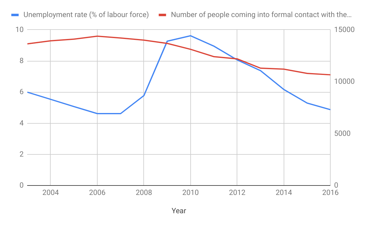
Some unemployed individuals may turn to crime, and this may be reflected in increased crime rates.
The graph below compares the United States unemployment rate as a percentage of the labour force with the number of people coming into formal contact with the police. It shows that the decrease in the unemployment rate after the 2008 financial crisis was associated with fewer people coming into formal contact with the police. Police contacts are not a measure of all crime, and this association alone does not establish that lower unemployment caused the decline.
(3) Increased stress levels and family breakdowns
Unemployment brings with it psychological costs. Higher stress levels, lower self-esteem, and increased mortality through illnesses are associated with increased unemployment. These are factors that can contribute to an increase in family breakdowns.
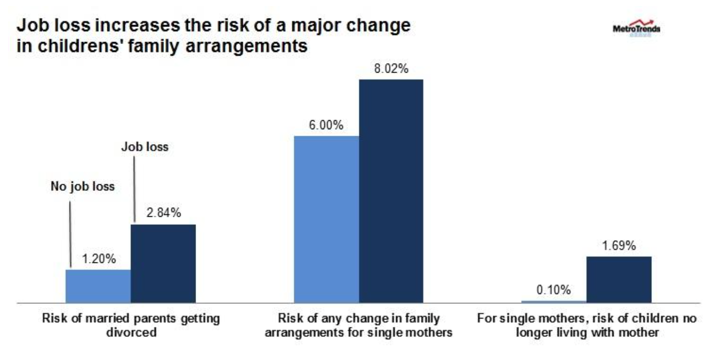
The Urban Institute is an economic and social policy research centre offering data on the well-being of people and places in the United States. A 2014 report by the Urban Institute found that for children with married parents, the risk of divorce doubles when a parent loses their job. The graph below summarises the data used in the report: it shows that job loss leads to an increase in the risk of change in family arrangements for single mothers from 6% to 8.02%, and that job loss for single mothers significantly increases the risk that their children will no longer live with them.
https://www.urban.org/urban-wire/lose-your-job-lose-your-family-how-unemployment-affects-family-stability
The report also found that unemployed parents are less likely to be married, meaning that family stability is lower in families with parents who have experienced unemployment.
Solutions for unemployment
Policies to decrease the natural rate of unemployment (The sum of frictional, structural and seasonal unemployment) can be classified into market-oriented and interventionist policies.
(1) Market-oriented policies
These policies seek to address factors that cause rigidities in the labour market. Removal of these factors will make it easier for labour demand and supply forces to determine the market wage-labour equilibrium:
(a) Lower minimum wage
Lower minimum wage can help to increase quantity demanded of labour. With more job opportunities available, fewer people shall be unemployed, reducing the extent of unemployment. However, this can have adverse effects for incumbent workers as their wage level might go down.
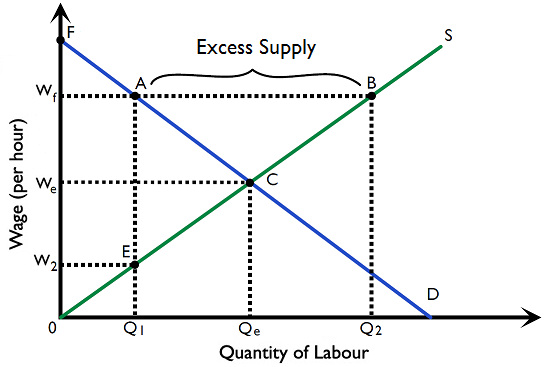
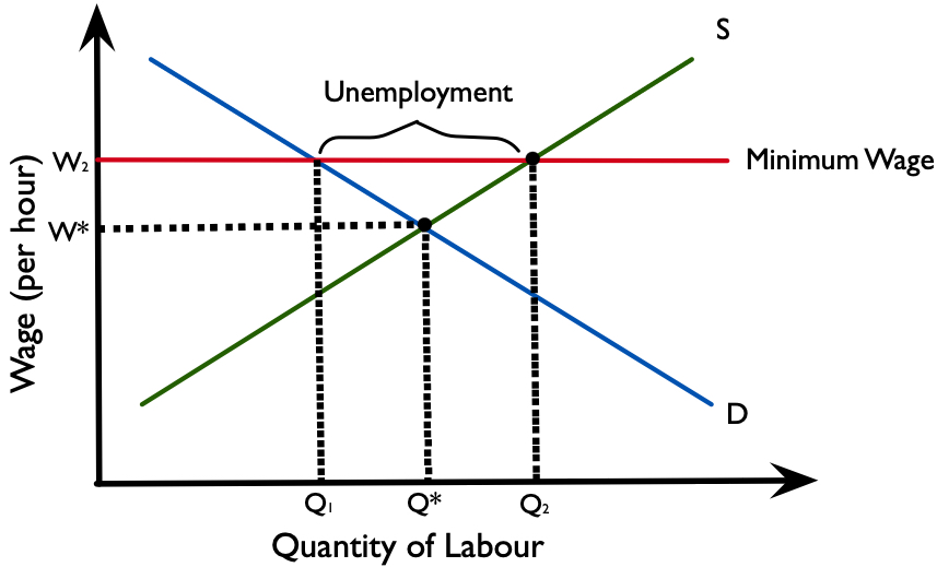
Figure 3.3.9 shows the impact of a minimum wage on structural unemployment. The labour market equilibrium is at \(W^*\) per hour. When the minimum wage of \(W_2\) is imposed, the quantity supplied of workers goes up, as there are more workers willing and able to work at \(Q_2\), but the quantity demanded for workers goes down to \(Q_1\), as employers want to hire fewer people at the higher wage rate. There is unemployment of \(Q_2 - Q_1\) at \(W_2\). If the minimum wage is lowered or removed, the quantity of workers employed shall increase.
(b) Lower unemployment benefits
The presence of unemployment benefits reduces the incentive for workers to take up jobs, especially low-paying jobs where wage levels may not exceed benefit levels. Lowering unemployment benefits can reduce frictional unemployment, but might lead to inadequate support for the unemployed. An alternative is to set a time limit for unemployment benefit claims, to give workers sufficient support when searching for a matching job.
(c) Reduced job security
Firms are reluctant to hire workers in the first place if it is difficult and costly to fire workers. Reducing job security by making it less costly to fire workers will make firms more willing to hire workers, especially young ones. This shall increase job opportunities and reduce the level of frictional unemployment.
(2) Interventionist policies
Interventionist policies attempt to influence the labour market by reducing non-market related barriers.
(a) Education and retraining
The government can encourage structurally unemployed workers to obtain skills that are more in demand. This could include the provision of training programmes, or give incentives for firms to hire and train these workers.
(b) Increase geographical mobility
The government may provide transport subsidies or low-cost housing to encourage structurally unemployed workers to take up jobs in other geographical locations.
(c) Improve the flow of information
The government can provide information about jobs in other geographical areas to structurally unemployed workers. It can also facilitate the flow of information between firms and job-seekers, via job centres or websites to reduce frictional and seasonal unemployment.
Policies to reduce demand-deficit/cyclical unemployment
Cyclical unemployment occurs because of the lack of aggregate demand in the economy. Policies to increase aggregate demand, including expansionary fiscal and monetary policies, can reduce cyclical unemployment. (Refer to Ch. 3.5 and 3.6 for details on expansionary fiscal and monetary policies.)
Low and stable rate of inflation
Inflation is the persistent increase in the general price level of all goods and services in an economy over a period of time.
Deflation is the persistent decrease in the general price level of all goods and services in an economy over a period of time.
- A one-off increase in price level does not constitute inflation. The price level must be increasing continuously over a period of time.
- An increase in the overall price level of goods and services is counted as inflation. One particular good becoming more expensive is not counted as inflation.
Calculating the rate of inflation/inflation rate
Inflation rate measures the percentage change in the general price level in relation to those in the previous period of time.
\( \dfrac{Price \; index \; in \; year \; n \; - \; Price \; index \; in \; previous \; year}{Price \; index \; in \; previous \; year} \times 100 \% \)
Change in inflation rate vs inflation rate
Change in the inflation rate is different from inflation rate: Change in inflation rate measures the change in inflation rate (%) over time, while inflation rate measures change in average price level over time. For example, the inflation rate was 5% in 2008-2009, and the inflation rate was 6% in 2009- 2010. We say that the change in the inflation rate was +1% between 2008-2009 and 2009-2010.
Disinflation means inflation rate decreases but the economy still involves a positive inflation rate. This differs from deflation, where there is a persistent decrease in the general price level. For example, if the inflation rate decreases from 4% in 2010-2011 to 2% in 2011-2012, there is disinflation but no deflation between the periods. This is because the price level is still increasing, even though the inflation rate is falling. If inflation decreases from 4% in 2010-2011 to -2% in 2011-2012, there is deflation. This is because the price level actually falls during the period. In addition, there is disinflation. This is because the inflation rate is falling during the period.
Measurement of the price level in an economy
Consumer price index is the measure of a weighted average price index of a market basket of consumer goods and services that a typical household consumes.
CPI assumes that typical households receive a certain bundle of household goods and services. Each household good receives a weighting based on the value contained in a market basket, and the change in the price level is tracked over time. The CPI assumes a base year with an index of 100.
Constructing a price index and calculating the rate of inflation
Table 2.3.4 Market basket of goods in country A in 2011 and 2012
| Goods | Amount in basket (A) | Price in 2011 (B) | Value of basket in 2011 (A×B) | Price in 2012 (C) | Value of basket in 2012 (A×C) |
|---|---|---|---|---|---|
| Beef | 10 | $15 | $150 | $14 | $140 |
| Beans | 37 | $3 | $111 | $4 | $148 |
| Chicken | 21 | $9 | $189 | $10 | $210 |
| Harps | 5 | $12 | $60 | $15 | $75 |
| Total | $510 | $573 |
To construct a price index, one has to first determine the basket of goods and the amount of each good to be included in the basket. This has to be kept constant over years in order to make comparisons. Also, a base (reference) year has to be chosen. The price index is calculated by:
\( Price \; index \; in \; year \; n = \frac{Value \; of \; basket \; in \; year \; n}{Value \; of \; basket \; in \; base \; year} \times 100 \)
Given the combination of goods in Table 2.3.4 and 2011 as the base year, the price index in 2011 and 2012 can be shown as follows:
\( Price \; index \; in \; 2011 = \frac{510}{510} \times 100 = 100 \)
\(\text{Price index in 2012}=\frac{573}{510}\times100\approx112.35\)
The price index in the base year will always be 100.
The rate of inflation can be calculated, using the equation below:
\( \frac{Price \; index \; in \; year \; n \; - \; Price \; index \; in \; previous \; year}{Price \; index \; in \; previous \; year} \times 100 \% \)
After obtaining the price index, the inflation rate (% change in price level) from 2011 to 2012 is calculated as:
\(\text{Inflation}=\frac{573-510}{510}\times100\%\approx12.35\%\)
The inflation rate between 2011 and 2012 is approximately 12.35%. Use the unrounded basket costs in the calculation, then round the final answer. A whole-number index of 112 would hide part of the increase.
Shortcomings with CPI
No measure of the price level is perfect, and problems with CPI should be noted:
(1) Upward inflation bias
Product quality changes over time. In the late 1990s, a high-end desktop would come with a 10GB hard drive, smaller in capacity than today's current desktop. Comparing computers from the 1990s and today while ignoring quality changes will overstate inflation. A phenomenon called outlet bias also exists. As prices increase, households that used to shop at high-end supermarkets may switch to wet markets, where goods are less expensive. Ignoring this, CPI also tends to overstate inflation.
(2) ‘Average household’
Different income earners may experience very different inflation rates from that stated by CPI if they have very different consumption patterns. For instance, a low-income household’s “basket of goods” may have a much higher proportion of food items than a typical household, and would experience much sharper inflation than the average household if the price level of food items increases.
(3) Volatility of CPI
CPI includes in its basket food items and petrol, which often experience swings in price. Economists wishing to study long-term trends of inflation want to eliminate these effects, and therefore a core (or underlying) inflation that leaves out food and petrol in the calculation is sometimes used.
(4) Data collection error
CPI figure is collected every month by a team of price collectors. Error in data collection might possibly occur in the process e.g. typing a wrong number for the price of a certain good.
Causes of inflation
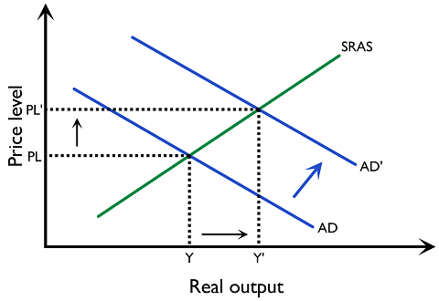
Demand-pull inflation is caused by an increase in aggregate demand (C + I + G + (X−M)) and can be shown in an AD-AS framework. In Figure 3.3.10, when \(AD\) increases to \(AD’\), both price level and real output increase from \(PL\) to \(PL’\) and from \(Y\) to \(Y’\) respectively.
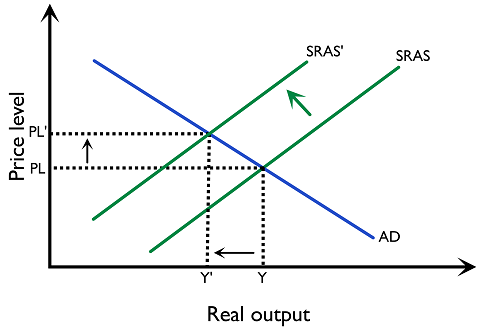
Cost-push inflation is caused by a reduction in aggregate supply. When factors of production become less readily available or more costly e.g. an increase in oil price, the \(SRAS\) curve shifts to the left to \(SRAS’\) and as a result, the price level increases from \(PL\) to \(PL’\), and real output level decreases from \(Y\) to \(Y’\) in Figure 3.3.11. This phenomenon is also known as stagflation.
Causes of deflation
Deflation can come about from improvements in the supply side of the economy and increased productivity. Figure 3.3.12 shows an outward shift in the LRAS leading to a lower price level.
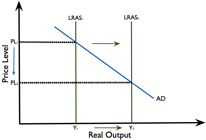
Deflation may also be the result of a fall in aggregate demand. In this case, it is a ‘bad’ thing. A fall in aggregate demand leads to a fall in the price level and a decrease in real output. This sort of ‘bad’ deflation will also lead to an increase in unemployment as firms need fewer workers if there is less demand.
The higher level of real output may also be associated with lower unemployment.
Consequences of inflation
(1) Redistribution effects
Inflation decreases the real purchasing power of cash. With the same amount of cash, fewer goods and services can be bought. Those who receive cash payments (e.g. pensioners, creditors, fixed income earner) and savers (those who save cash) suffer from inflation because of their real purchasing power with the same amount of cash decreases.
(2) Uncertainty
With a high and unstable inflation level, firms become more cautious about making future plans and are reluctant to invest, hampering economic growth.
(3) Less savings
People tend to spend more rather than save if they foresee a decrease in the value of funds from savings due to inflation. This has a negative effect on the supply of savings for investment purposes.
(4) Loss of international competitiveness
With inflation, a country’s exports become more expensive in the international market. This adversely affects international competitiveness, as trading partners shift to domestically produced substitutes or other countries’ imports.
(5) Inefficient allocation of resources
Inflation distorts the price mechanism: a rise in average prices means that the price mechanism cannot act as a resource-allocating mechanism. Resource allocation depends on prices rising and falling to provide information about demand, but if average prices are rising continuously allocation is distorted.
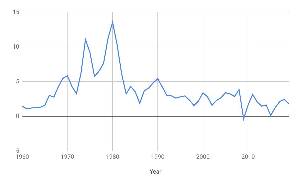
The United States experienced a period of high inflation in the 1970s, as shown in the graph below.
Redistribution effects
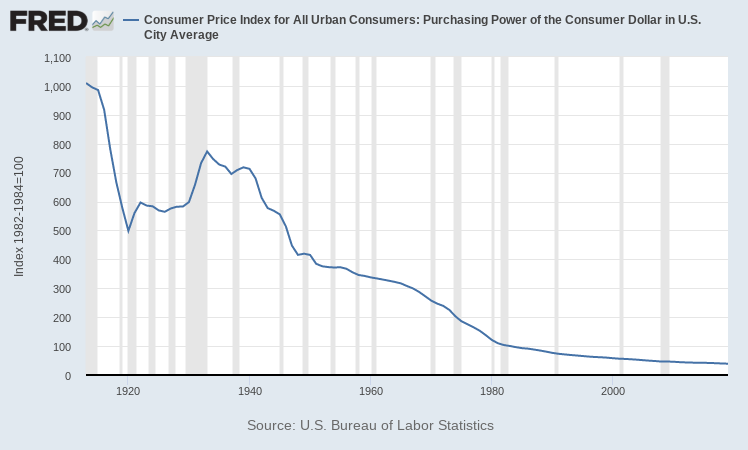
This high inflation led to a fall in the purchasing power of the dollar. The below graph shows the steep drop in the purchasing power of the dollar in the 1970s. The purchasing power of the dollar indicates how much each consumer can buy with the same amount of cash; the steep decrease in the dollar’s purchasing power in the 1970s, therefore, indicates that the amount that consumers were able to purchase was also decreasing.
Uncertainty
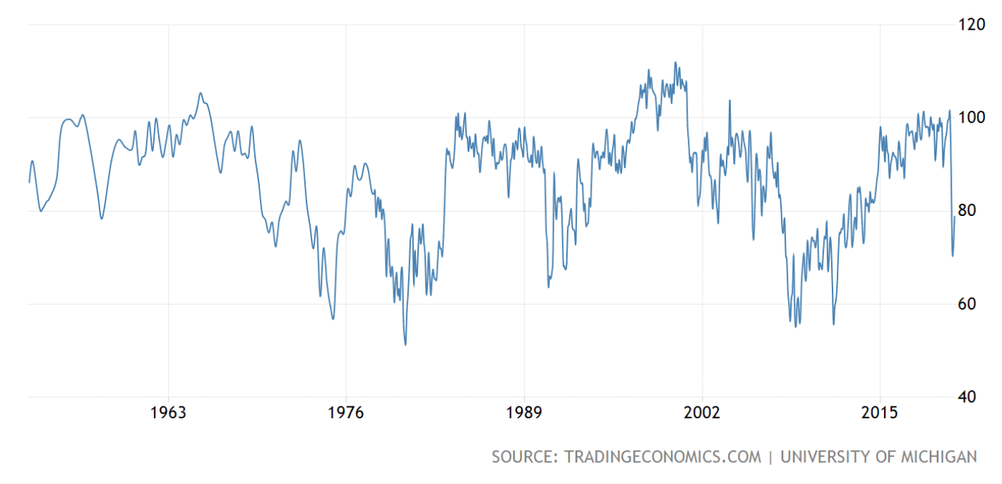
The Index of Consumer Expectations focuses on how consumers view prospects for their own financial situation and how they view the prospects of the general economy in the short and long term. The graph below shows that there was a sharp decrease in the index in the 1970s, concurrent with the rise in inflation.
Loss of international competitiveness
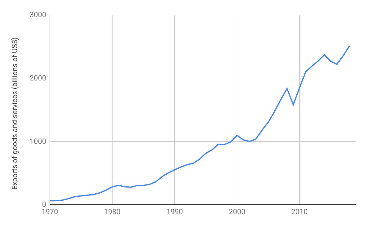
The graph shows US exports of goods and services in current US dollars, not constant 2020 dollars. These nominal values reflect changes in prices as well as quantities. A lower dollar value in the 1970s does not, on its own, show weaker international competitiveness; relative prices, exchange rates and export volumes would also need to be considered.
Consequences of deflation
(1) Redistribution effects
Deflation benefits those who receive cash payments or hold cash because the real purchasing power of cash increases with deflation. For instance, fixed income earners and creditors gain, while borrowers and payers of fixed income suffer.
(2) Deflationary spiral and high levels of cyclical unemployment
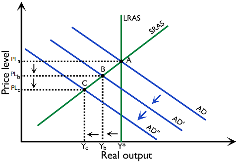
Deflation may set off events that have the effect of worsening deflation even further, thus we call it a deflationary spiral. Expecting lower prices, firms decrease production and investment. Consumers also reduce consumption in expectation of lower prices. All of these lead to a continuous decrease in aggregate demand, which leads to a lower level of prices and economic output. As seen in Figure 3.3.14, there are successive falls in the AD, from \(AD\) to \(AD’\) and \(AD’’\). The continuous reduction in aggregate demand will result in demand-deficient unemployment, also known as cyclical unemployment.
(3) Bankruptcies
Firms may have to default on their debts due to the combined effects of lower aggregate demand and higher real debt. The fall in the value of assets that firms and households own also make it more difficult to use the assets as collateral to borrow, which increases the risk of bankruptcy.
(4) Deferred consumption
If prices are falling, consumers are likely to put off the purchase of expensive goods, such as durable goods, as they want to wait until the prices drop further. This can lead to a fall in aggregate demand and a deflationary spiral.
(5) Increase in the real value of debt
Deflation raises the real burden of a fixed nominal debt. As the price level falls, money’s purchasing power rises, so the amount owed represents more goods and services. Repayment can also become more difficult if the borrower’s nominal income falls.
(6) Inefficient resource allocation
Resource allocation depends on prices rising and falling to provide information about demand, but if average prices are falling continuously allocation is distorted. Therefore, deflation means that the price mechanism cannot act as a resource-allocating mechanism.
(7) Policy ineffectiveness
The low interest rates associated with deflation make monetary policy ineffective as it is not possible to reduce interest rates further to increase aggregate demand.
Japan’s asset-price bubble collapsed in the early 1990s. Persistent consumer-price deflation emerged later, in the late 1990s; the entire period from 1991 to 2001 should not be described as continuous deflation.
Redistribution effects and an increase in the real value of debt leading to bankruptcies
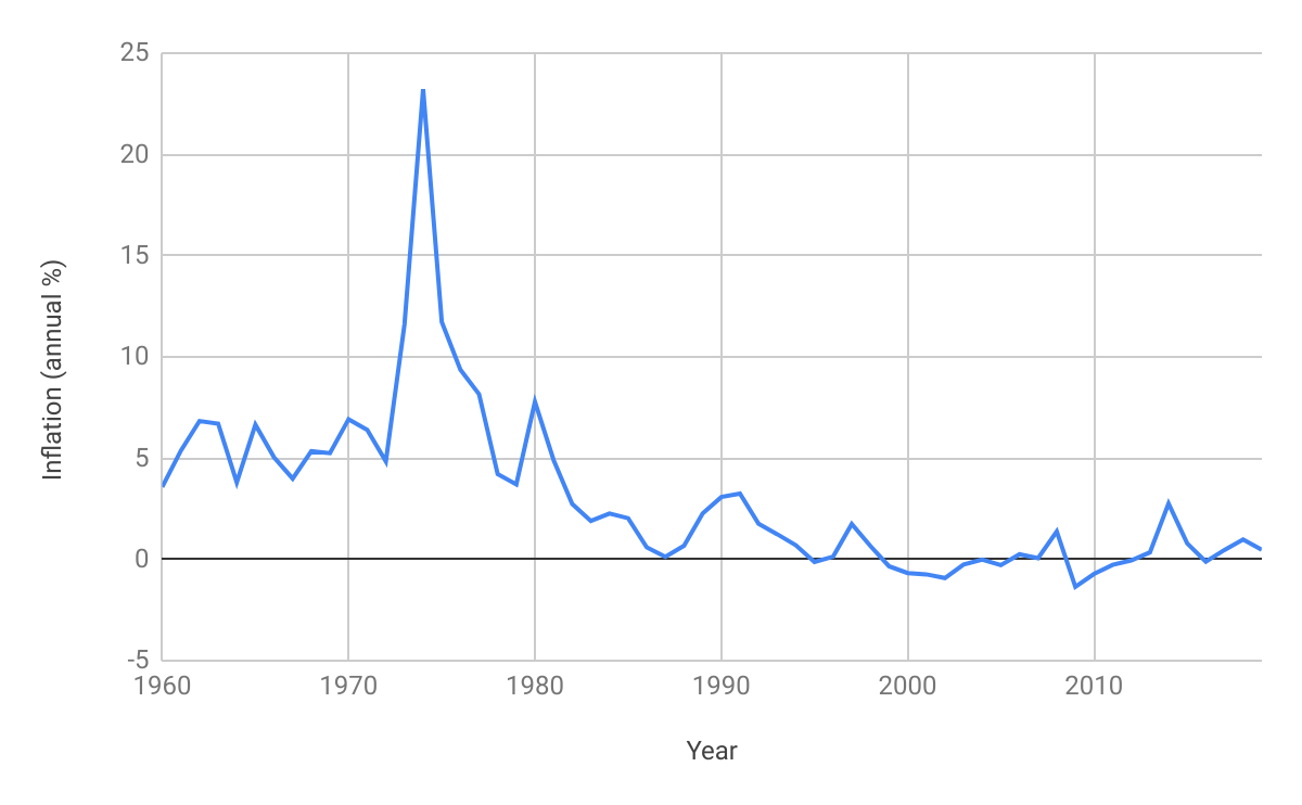
A fixed nominal debt becomes more burdensome when the price level is lower than expected. For a given nominal repayment, real debt = nominal repayment ÷ price index. Its proportional increase relative to the expected burden is therefore (expected price index ÷ actual price index) − 1. A quoted nominal bond yield of 2.1% in 1997 does not by itself establish a 20% unexpected increase in the debt burden by 2007: the expected and actual price paths, and the loan terms, would also be needed.
A 2003 report by the International Monetary Fund argued that this redistribution of wealth led to households and firms which had high levels of debt limiting their spending and investment, and higher rates of bankruptcy among such households and firms.
Deflationary spiral and high levels of cyclical unemployment
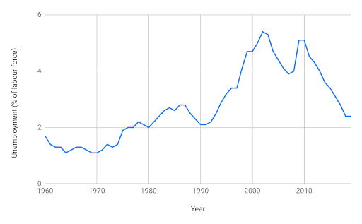
The graph shows Japan’s unemployment rate between 1960 and 2019. Unemployment rose sharply between 1990 and 2002, spanning the post-bubble slowdown and the later emergence of persistent deflation.
This rise in the unemployment rate is likely in part due to sticky wages in Japan. When wages are ‘sticky’, they do not respond quickly to changes in the labour market; for example, while we might expect an increase in the demand for labour to lead to an increase in the wage rate, ‘sticky’ wages mean that the wage rate might remain low despite the increase in demand.
Sticky wages meant that firms were more inclined to lay off workers in response to deflation, rather than having to make large nominal wage cuts.
Deferred consumption
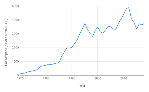
The graph reports Japan’s consumption from 1970 to 2019 in current US dollars. Both domestic prices and the yen–dollar exchange rate affect this series, so changes in the plotted values cannot be read directly as changes in real consumption. The graph alone does not establish that consumers postponed purchases because of deflation.
Policy ineffectiveness
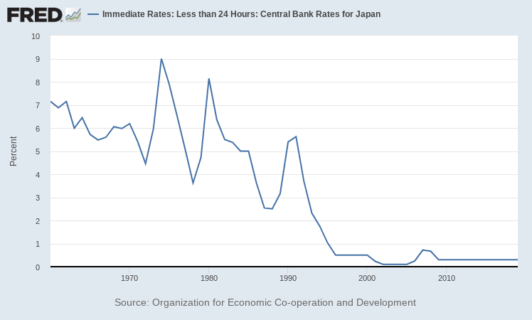
Japan’s deflation has meant that its monetary policy has been constrained by the Zero Lower Bound (ZLB) on interest rates. The ZLB occurs when the interest rate is at or near zero, which means that the central bank cannot reduce it further in order to stimulate economic growth.
The graph below shows Japan’s interest rate between 1960 and 2019. The fact that the interest rate was around 0.5% from 1995 onwards indicates that the central bank’s ability to lower the interest rate in order to stimulate consumption and investment and therefore boost the inflation and economic growth rates was limited.
Policies to address inflationary pressure
As seen in the previous section, demand-pull and cost-push inflation require very different policy solutions. Therefore, identifying the root cause of inflation is important for correct policy prescription, and wrong policy solutions can create more harm than good.
To combat demand-pull inflation, contractionary fiscal and monetary policies can be used to reverse the increase in aggregate demand.
(1) Reduce government spending
Governments can reduce government spending to reduce AD, for example, by cutting spending on infrastructure. However, such measures might be politically unpopular and may hamper the long-term productive capacity of the economy.
(2) Increase taxation
Governments can increase taxes, causing a reduction in households’ disposable income and firms’ retained profits. This causes consumption and investment expenditure to fall, leading to a lower AD.
(3) Increase interest rates
The central bank may also increase interest rates to dampen investment and consumption expenditure. The effects of the latter are especially pronounced in economies with a high number of homeowners with mortgages. To combat cost-push inflation, governments can use supply-side policies to increase aggregate supply.
(4) Supply-side policies
In the energy crises of the 1970s, a number of events adversely affected the supply of oil by the Organization of Petroleum Exporting Countries (OPEC) members. As oil is a major factor of production, this leads to a decrease in SRAS and cost-push inflation. The response to this has been an increase in energy exploration by developed countries, and the development of new, fuel-efficient technology. These are policies that can reduce dependency on imported oil, but typically takes a longer period of time. If the issue is coming from the labour market, policy-makers may attempt to lower the minimum wage or curb union power to increase the flexibility of the labour market or encourage immigration to increase labour supply. However, these measures tend to also increase income inequality, as wage workers are in a worse position to negotiate wages.
Sustainable level of government (national) debt
Government debt is the accumulation of all the government’s budget deficits, and it represents the total amount of money that the government owes to its creditors.
We measure government debt as a proportion of GDP in order to understand the proportion of national output that the government owes.
Costs of a high level of government debt
Although there may be short-term benefits of high government spending, as it drives economic growth, there will be long-term costs associated with the increasing amount of government debt.
1) Debt servicing costs
Debt servicing is the money required to make payments on the principal and interest on a loan in a given time period. When government debt increases, debt servicing costs increase, and the government has to spend more of its budget on interest costs. This might have adverse effects:
- It might lead to crowding out of public investments, as the government monopolises the funds available in the economy for borrowing and does not leave firms with enough access to funds for investment.
- The government might have to decrease spending in other areas in order to be able to afford its interest repayments.
- If the government chooses to not decrease its spending in other areas, it will have to increase taxes; this, in turn, might lead to falling output.
- The government might have less ability to respond to emergencies, as governments often have to borrow money to do so and if the debt is already too big, the government will have few options available.
2) Impact on the government’s credit rating
Credit rating reflects the risk and return associated with different investments, and credit rating agencies give countries credit ratings based on the risk of investing in that country, and advise financial investors about where to put their money by considering the credit ratings.
If a country has a high level of government debt, the credit ratings agencies may downgrade its credit rating. This would adversely impact the country’s ability to attract investment.
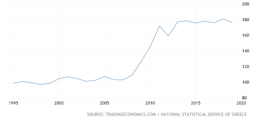
The graph below shows the ratio of Greece’s government debt to GDP from 1995 to 2020. It shows that the government debt to GDP ratio increased sharply from 2007 onwards, to a high of around 176.60% of GDP in 2019.
Debt servicing costs
‘Amortisation’ refers to the process of paying off debt. The graph below shows an estimate of Greece’s amortisation costs over time from CEPS, a think-tank which focuses on EU affairs.
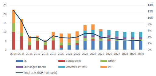
The CEPS estimates show that the costs of repaying Greece’s government debt could be as high as 8% of total GDP in 2023 and 2024. This suggests that the Greek government would have to significantly reduce expenditure in other areas in order to be able to service its debt.
Impact on the government’s credit rating
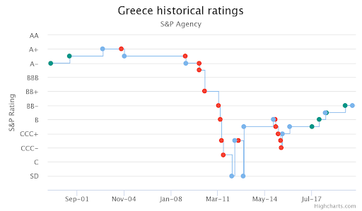
The graph below shows Greece’s credit rating over time, as reported by Standard & Poor’s, an American credit rating agency.
The increase in Greece’s government debt burden was associated with a steep drop in its credit rating, from A- in early 2008 to C in early 2011. This low credit rating negatively impacted Greece’s impact to attract inward investment, therefore limiting its recovery from the Eurozone debt crisis of 2009.
Potential conflict between macroeconomic objectives
1) Low unemployment and low inflation
We can assume that there might be a trade-off between achieving the macroeconomic objectives of low unemployment and low inflation simultaneously. When unemployment falls, it can put upward pressure on wages, leading to inflation.
The Phillips curve shows the relationship between inflation rate and unemployment rate.
Short-run Phillips curve
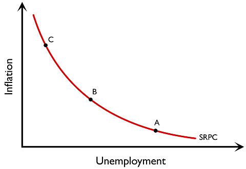
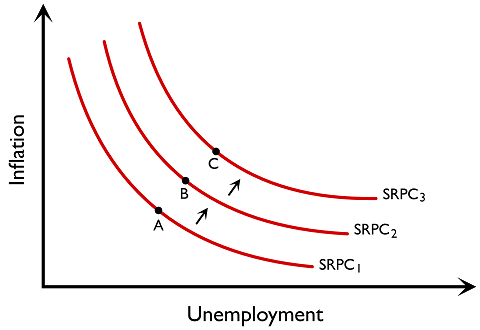
The short-run Phillips curve shows an inverse relationship between inflation and unemployment rate, suggesting that possible trade-off can be made between inflation and unemployment.
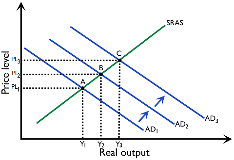
The reason behind the short-run Phillips curve can be explained using the AD-AS model. Assume that the macro equilibrium starts at A. An increase in the AD from \(AD_1\) to \(AD_2\) moves the economy to \(B\), and a further increase of AD from \(AD_2\) to \(AD_3\) moves the economy to \(C\).
Movement from \(A\) to \(B\), as well as from \(B\) to \(C\), is associated with higher prices and output levels. As the output level increases, unemployment falls. (Figure 3.3.14)
If we correspond each point \((A, B, C)\) on the AD-AS model to the Phillips curve, point \(B\) has to be to the upper left-hand corner of \(A\), and point \(C\) has to be to the upper left-hand corner of \(A\) and \(B\) in order to show that price level increases and the unemployment rate falls as AD increases. Linking point \(A\), \(B\) and \(C\) together in Figure 3.3.15 gives us the short-run Phillips curve.
The shift of short-run Phillips curve
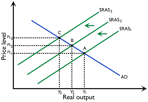
A shift in SRAS will cause a shift in the short-run Phillips curve. In the 1970s, the oil shocks caused the cost of production of goods and services to increase. This can be represented by a shift of SRAS from \(SRAS_1\) to \(SRAS_2\), or from \(SRAS_2\) to \(SRAS_3\). Macro equilibrium moves from \(A\) to \(B\) or from \(B\) to \(C\) in Figure 3.3.16. Price level increases and output level reduces, causing a higher level of unemployment. This phenomenon is known as stagflation.
If we correspond point \(A\), \(B\) and \(C\) on the AD-AS model to the Phillips curve, we find that the phenomena can be explained by an outward shift of the short-run Phillips curve. (Figure 3.3.17)
Long run Phillips curve
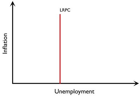
The long-run Phillips curve shows that there is no trade-off between inflation and unemployment. The long-run Phillips curve is vertical at the full employment level, or the natural rate of unemployment.
The natural rate of unemployment (NRU) is the component of total unemployment not influenced by the demand side and is therefore non-cyclical in nature. NRU includes frictional, seasonal and structural unemployment.
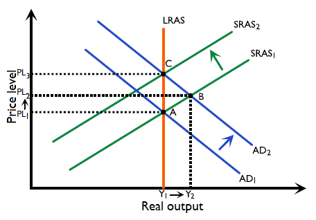
Assume that the macroeconomic equilibrium is at point \(A\). If there is an increase in AD, the price level increases from \(PL_1\) to \(PL_2\) and the real output level increases from \(Y_1\) to \(Y_2\), as indicated at point \(B\). If workers receive a fixed income, workers shall realise that the real purchasing power of their income is eroded by an increase in the general price level. In the long run, as factor costs are flexible, e.g. employment contracts can be renegotiated, workers will demand an increase in nominal wages to maintain its original level of purchasing power. This is shown by the shift in the \(SRAS\) from \(SRAS_1\) to \(SRAS_2\). The macroeconomic equilibrium now goes to point \(C\). In the long run, as the factor cost is always flexible, the monetarist suggests that the macroeconomic equilibrium will always be restored at the LRAS level. (Figure 3.3.18)
Therefore, if we translate the idea that the long run macroeconomic equilibrium is always at the LRAS level on the long-run Phillips curve, the long-run Phillips curve shall be a straight line, showing that there is no trade-off between inflation and unemployment. The economy shall always produce at the natural rate of unemployment level. (Figure 3.3.19)
Nominal wage refers to wage not adjusted for inflation. Real wage refers to wage adjusted for inflation and reflects real purchasing power.
2) High economic growth and low inflation
When there is rapid economic growth, it is likely that inflationary pressures will increase; this is particularly likely when growth is above the long-run trend rate, and AD increases faster than AS.
When the economy grows quickly, firms have difficulty employing enough labour; wages are likely to go up as firms compete over scarce labour, increasing firms’ costs of production and leading to higher prices. Furthermore, if the aggregate demand is growing faster than the aggregate supply, the overall price level will increase.
This can be seen in Figure 3.3.20, where the increase in economic growth (indicated by the shift out of the AD curve) leads to an increase in inflation from PL to PL’.
3) High economic growth and environmental sustainability
High levels of economic growth may harm the environment. Increases in output usually involve the use of more non-renewable resources, and more damage to the environment resulting from increased pollution. For example, if the economy grows and supplies more manufactured goods, the emissions from factories which produce manufactured goods will increase.
However, there is not necessarily a tradeoff between economic growth and sustainability, as economic growth can be achieved in a sustainable manner. For example, emissions could be kept low by using renewable energy such as solar or wind power to achieve economic growth.
4) High economic growth and equity in income distribution
The returns to economic growth are not always distributed evenly. If economic growth causes a relatively higher increase in income level for the rich than the poor, then the income gap widens and income inequality increases. However, if the harvest from economic growth can be distributed evenly across all levels of society, then income distribution can be improved.