3.2 Variations in economic activity - aggregate demand and aggregate supply
Aggregate demand
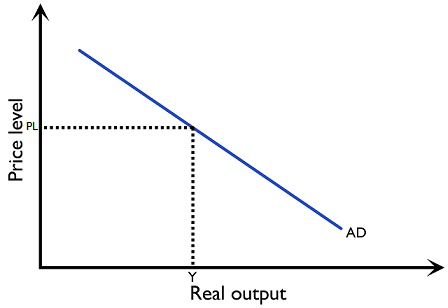
Aggregate demand (AD) shows the total spending on domestic goods and services at various price levels in an economy over a period of time. Total spending consists of C + I + G + (X – M).
Factors causing changes in consumption expenditure
Consumption expenditure is the total spending by consumers on domestic goods and services. Consumers spend on durable goods, like cars, and non-durable goods, like toilet paper, which are used up over time. The following are the key determinants of the consumption expenditure:
(1) Consumer confidence
Consumers are likely to spend more if they are optimistic about the future economy and their future incomes.
(2) Interest rate
Some consumer expenditure is financed on credit, especially purchases of durables. When the interest rate decreases, the cost of borrowing falls, therefore increasing consumption. In addition, a lower interest rate reduces returns to savings. Consumers will save less and increase consumption.
(3) Wealth
When households have more assets (or the value of their existing assets, such as property, bonds, and stocks increase), they are willing to spend more on consumption.
(4) Personal income taxes
Households’ disposable income (i.e. post-tax income) increases if tax rates are decreased. This leads to an increase in consumption expenditure.
(5) Level of household indebtedness
Consumption can be financed from loans in addition to income. Indebtedness refers to the amount of past loans households have taken. If indebtedness is high, households will need to use a higher portion of their income to service debt, reducing consumption expenditure.
(6) Expectations of the future price level
If consumers expect the future price level to increase, they will increase spending now, especially on durable goods. If they expect the price level to fall, they will put off their consumption as goods will be less expensive in the future.
Factors causing changes in investment expenditure
Investment expenditure is the addition of capital stock to the economy by firms. This includes replacement investment, where firms invest to maintain the productivity of their current capital, and induced investment, where firms invest to increase their output. Investment expenditure is by far the most volatile component of GDP. When a recession occurs in an economy, the decrease in investments often make up the largest part of the recession. The followings are the key determinants of the investment expenditure:
(1) Interest rate
Investments from firms are often financed through loans. A decrease in the interest rate reduces the cost of borrowing and increases investment expenditure.
(2) Business confidence
Firms have to decide in advance whether to invest in their production capacity to meet future demand. Such decisions are based on limited information about the future, and expectations play an important role in investment decision making. If firms expect the economy to perform well, investment expenditure increases.
(3) Technology
Development of new technology can spur new investment. For instance, such has been the case with solar power in recent years.
(4) Business taxes
The level of business taxes affects firms’ post-tax profits, which in turn affects firms’ incentive to invest. Lower business taxes induce firms to invest more.
(5) Corporate indebtedness
When corporate indebtedness is high, firms will need to use a higher portion of income to service debt, reducing investment expenditure.
Factors causing changes in government expenditure
Government expenditure includes health, education, housing, and defence. Note that it does not include transfer payments, such as unemployment benefits and subsidies, as these do not represent the purchase of goods and services. The following is the key determinant of government spending:
1) The government’s economic and political priorities
How much the government spends depends on its political and economic priorities. For example, if the government wants to improve education, this will require additional spending on building schools and hiring teachers.
Factors causing changes in net exports
Net exports is the difference between expenditure on exports, which are the domestic goods and services bought by foreigners, and expenditure on imports, which are goods and services bought by domestic consumers from foreign firms. The followings are the key determinants of net exports:
(1) Income of trading partners
When the income levels of trading partners increase, this will lead to an increase in demand for domestic exports. For example, when the incomes of Canadian residents rise, their demand for imports from the USA is likely to rise.
(2) Exchange rate
The exchange rate is the price of one currency in terms of another currency. If the domestic currency strengthens, it becomes more expensive in relation to foreign currency. Ceteris paribus, domestically produced goods become more expensive while imported goods become relatively cheap. This lowers the quantity demanded for domestic exports and increases the quantity demanded for imports. Assuming that PED for exports and imports is elastic, total export revenue would fall and total import expenditure would increase. This causes the domestic net export value (X-M) to decrease.
(3) Change in trade policies
Trade barriers imposed by economies decrease the level of trade. If the country decides to adopt a free trade policy, it might reduce tariffs and allow for more imports and exports. If it decides to adopt a protectionist policy, the level of imports and exports will drop.
Shifts of the AD curve caused by changes in its determinants
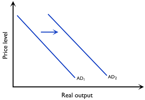
As AD is composed of C + I + G + (X – M), any non-average price level factors that cause a change in these components will lead to a shift in the aggregate demand curve, as seen in Figure 3.2.2:
Short-run Aggregate Supply (SRAS)
Aggregate supply is the total quantity of domestic goods and services produced in an economy at different price levels over a certain time period, ceteris paribus.
Aggregate supply is concerned with the production side of the economy and a distinction is made between short-run and long-run aggregate supply. In the short-run aggregate supply, the costs of the factors of production are kept constant, while they are flexible in the long-run.
Reasons for the positive slope of the short-run aggregate supply curve
A short-run aggregate supply curve (SRAS) has a positive slope, as shown in Figure 3.2.3. The shape of the slope can be explained by how a change in the price level would change the firm’s profitability and hence output level.
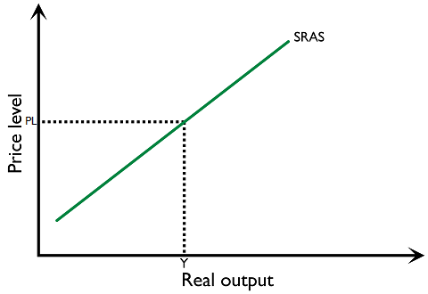
In the short run, resource prices e.g. wages are assumed to be constant. This is because the wage is sticky (i.e. wage contracts between firms and workers are often signed for a certain period of time, and the nominal wages remain constant during this period). In addition, employees might not realise the higher price has affected their purchasing power, so employees are slow to adjust to the nominal wage level.
When the average price level increases and the resource price level is held constant, firms’ profitability increases and firms increase output level.
Shifts of the SRAS curve
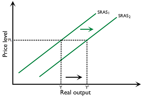
A short-run aggregate supply curve can be shifted by non-price factors. When the SRAS curve shifts towards the right at a given price level, real output increases from \(Y\) to \(Y’\). (Figure 3.2.4)
The following factors are factors causing a shift of the SRAS curve
(1) Change in resource prices
A decrease in resource prices shifts the SRAS curve to the right, and each price level corresponds to a higher output level produced.
(2) Change in business taxes and subsidies
Taxes and subsidies affect the profits of a firm. With lower taxes or higher subsidies, the cost of production decreases. The SRAS curve shifts to the right. Firms supply more output at every price level.
(3) Supply shock
When the availability of raw materials or other productive resources become restricted, prices of raw materials increase, increasing the costs of production to firms. The SRAS curve shifts to the left.
Alternative views of aggregate supply
In AD-AS theory, there is the debate about the shape of the long-run aggregate supply curve. There are two opposing views on the long run AS curve –the monetarist/neo-classical view and the Keynesian view.
Monetarist/neo-classical view
The monetarist makes the following assumptions about the market in the long run:
- Factor markets and good markets are flexible
- When the price level changes, factor costs change to reflect these changes fully
In the long run, assuming that the price level increases, factor costs would also increase (due to the assumption of wage flexibility) to match the increase in prices. Firms’ profitability remains constant and hence changes in the price level have no impact on the level of output supplied. In the long run, the aggregate supply curve is vertical, as shown in Figure 3.2.5.
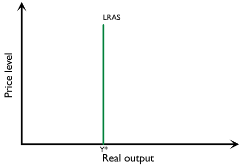
The real output level Y* to which the neoclassical long-run AS corresponds is called the potential level of output. It is the output level at which the economy only experiences a natural rate of unemployment. A reduction in the natural rate of unemployment can shift LRAS to the right.
Keynesian view
Keynes makes the following assumptions about the market in the long run:
- Wage and price stickiness: it is easy to raise prices and wages, but much harder to adjust them downwards
- At times of deep recession, even if workers are willing to take lower wages, they may not necessarily get employed because the business sentiment is poor and firms expect low aggregate demand
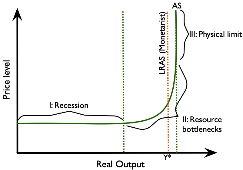
Keynesian economics is sometimes called recession economics, and the shape of the Keynesian aggregate supply curve makes a distinction in the economy while in recession and full employment, as shown in Figure 3.2.6. There are three sections on the Keynesian AS:
I: Recession (flat-slope long-run AS)
Recession means two or more consecutive quarters of negative economic growth. When there are a lot of unused resources and capacity in the economy, even if firms try to employ more resources to increase production, the costs of the factors of production do not increase because the market has many unemployed workers that are readily available.
II. Resource bottlenecks (upward-sloping AS)
As the economy moves away from recession and increases its outputs, it becomes increasingly difficult to employ resources in the economy. While some resources are still abundant when production increases, there are bottlenecks in other resources. While it is still possible to increase production, factor prices are bid up when there are bottlenecks, increasing the overall price level. Therefore the AS is upward sloping: price level and national income are positively related.
III. Full capacity (vertical long-run AS)
At the vertical section of the Keynesian AS curve, the economy has reached its full-employment or potential level of output. There is no spare productive capacity available for a sustained increase in output. Further increases in aggregate demand raise the price level rather than real output.
Full employment does not mean 0% unemployment. Frictional and structural unemployment can remain when output is at its potential level. Both the vertical Keynesian AS section and the neoclassical LRAS represent a capacity constraint; the distinction between the models concerns adjustment and the possibility of persistent spare capacity, not an assumption that the Keynesian limit lies beyond full employment with every worker employed.
Shifts of the AS curve over the long-run (monetarist/neo-classical LRAS) or over the long term (Keynesian AS)
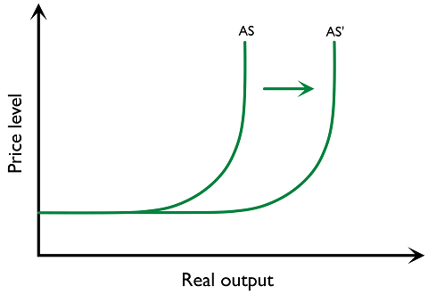
Recall that an economy’s aggregate supply curve is related to its productive factors (labour, capital, land and entrepreneurship). When there is an improvement in the economy’s productive capacity, the long-run aggregate supply curve shifts outward, like the expansion of the economy’s production possibilities frontier. The shifting of the monetarist and Keynesian aggregate supply curve may look different, but both represent an expansion in the productive capacity, as seen in Figure 3.2.7 and Figure 3.2.8.
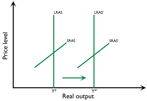
- The short-run aggregate supply changes together with the long-run AS under the monetarist view. The short-run aggregate supply shall be labelled as SRAS while the long-run should be labelled as LRAS.
- The long-run aggregate supply curve shall be labelled AS under Keynes’ perspective, as Keynes did not deliberately distinguish the short run and long run concept in his works.
(1) Improvement in efficiency
When there is better organisation of productive factors or reduced wastage, the existing quantity of resources can produce more output.
(2) New technology
With new technology, a higher quantity of output can be produced with the economy’s existing productive resources. This increases the economy’s productive potential.
(3) Increase in the quantity or quality of factors of production
This may include the discovery of new raw materials (such as energy resources), or an increase in population, or improvement in the education level of the workforce.
(4) Institutional factors
A variety of institutional factors, such as the introduction of bureaucratic red tape, make employment of resources more difficult and less efficient and could reduce production capacity.
Macroeconomic Equilibrium
Short-run macroeconomic equilibrium
The macroeconomic equilibrium is determined by the intersection of the AD and SRAS/AS, where the aggregate level of output demanded by various agents is matched by the supply-side of the economy (Figure 3.2.9). It also reflects the level of employment in the economy; labour being one of the factors of production, when output increases, there is generally an increase in employment.
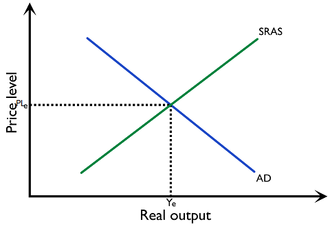
Any shift in AS and/or AD will change the macro equilibrium. Four cases of change in the AD and AS are explored. Students are expected to know the direction of change in price and real output levels, as well as the associated AD-AS diagrams. (Table 3.2.10)
Table 3.2.10 Shifts in short-run AS and AD curves
| Short-run AS | AD | |||
|---|---|---|---|---|
| 1. Increase
(rightward shift) |
2. Decrease
(leftward shift) |
3. Increase
(rightward shift) |
4. Decrease (leftward shift) |
|
| Example(s) | Favourable productivity shock | Negative productivity shock, stagflation | Expansionary fiscal/monetary policy, optimism | Contractionary fiscal/monetary policy, pessimism |
| Price level | \( \downarrow \)
|
\( \uparrow \) | \( \uparrow \) | \( \downarrow \) |
| Real output level and employment | \( \uparrow \) | \( \downarrow \) | \( \uparrow \) | \( \downarrow \) |
Long-run equilibrium: monetarist/neoclassical model
In the neoclassical view, all factor markets are flexible. Therefore the macroeconomic equilibrium will always be at the potential output level. This can be illustrated in Figure 3.2.11.
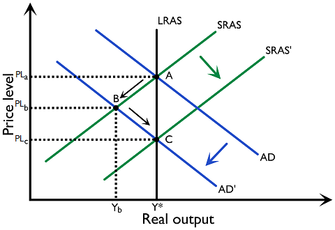
Assume that the economy is originally at point A. Consider a shock in AD that decreases the aggregate demand from AD to AD’. Neo-classical economists assume that the economy will move automatically to its long-run equilibrium. The short-run equilibrium changes from A to B, real output decreases from \(Y^*\) (the potential output level) to \(Y_b\), and the price level decreases from \(PL_a\) to \(PL_b\). In the long run, the factor market is flexible. As the price level drops, employees’ real wage increases. Employers might negotiate down the nominal wage in view of the current level of unemployment. The cost of production decreases. The short-run aggregate supply shifts from SRAS to SRAS’.
The macro equilibrium moves from \(B\) to \(C\). Price level reduces from \(PL_b\) to \(PL_c\) and real output is restored at the potential output level \(Y^*\). Therefore, the long run macro equilibrium always stays along the LRAS output level \(Y^*\).
In the neo-classical model, the impact of changes in aggregate demand will be on the price level only. As can be seen in Figure 3.2.11, the shifts in AD do not change the real level of output when the economy is on the LRAS. Any increase in aggregate demand will be purely inflationary in the long run, so there is no role for the government to play in trying to steer the economy towards full employment. There is no role for government intervention, and the economy should be managed by market forces.
Long-run equilibrium: Keynesian model
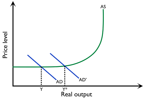
In the Keynesian model, the long run equilibrium output level is determined by the intersection of the AD and AS curves. The long run equilibrium output level is not necessarily equal to the level associated with “full employment” as suggested by the monetarist model. Instead, the equilibrium level of output can occur at different levels of output, and depends on the level of aggregate demand in the economy. This means that the economy can be in long-run equilibrium at a level of output which is below the full employment level of national income.
In the Keynesian view, AD can increase such that there is an increase in the level of real output without any increase in the price level, as shown in Figure 3.2.12.
Representing different economic states using the neoclassical and Keynesian AD/AS model
Recessionary gap
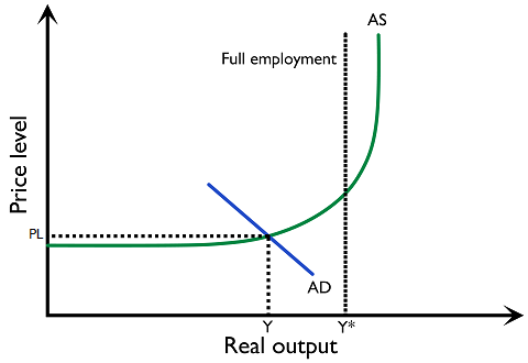
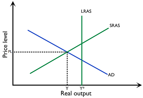
Whenever AD intersects with AS/SRAS at an output level less than the full employment level \(Y^*\), there is a recessionary or deflationary gap, as shown in Figure 3.2.13.1 and 3.2.13.2. Recessionary/deflationary gaps will occur when the actual output level \(Y\) is lower than the full employment level output at \(Y^*\).
Inflationary gap
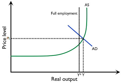
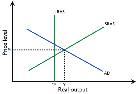
Whenever AD intersects with SRAS/AS at an output level more than the full employment level \(Y^*\), there is an inflationary gap, as shown in Figure 3.2.14.1 and 3.2.14.2. Inflationary gaps occurs, when the actual output level \(Y\) is higher than the full employment level output at \(Y^*\). .