2.7 Role of government in microeconomics
Reasons for government intervention in markets
Governments might intervene in the market for several reasons. These include
1) earning government revenue through taxation
2) supporting firms or households on low incomes through subsidies or benefits
3) influencing the levels of production and consumption
4) correcting market failure
5) promoting goals like sustainability and equity.
Main forms of government intervention in markets
Price controls: price ceilings and price floors
A 'price control' is a price that is set above or below the market equilibrium by the government. Price controls result in shortages or surpluses of goods.
A 'price ceiling', or maximum price, is the setting of the market price lower than the market equilibrium by the government, meaning that no seller can sell the good at a price higher than the maximum price.
The government imposes a price ceiling for several reasons:
- To protect the buyers so that lower-income households can also afford the good or service. Examples are food price controls and rent controls.
- To lower the price of goods that are unreasonably high.
Figure 2.7.1 shows the effects of a price ceiling on the market. An effective price ceiling has to be set below the equilibrium price Pe. When the price ceiling of Pc is imposed, the price is lowered from Pe to Pc; the producer is only willing and able to supply at Q1 while consumers are willing and able to buy at Q2. A shortage of (Q2-Q1) units exists at the price Pc. At Pc, the quantity transacted decreases from Qe to Q1.
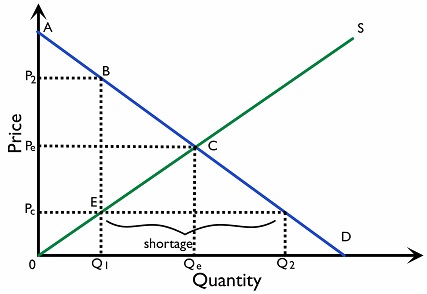
The impact of a price ceiling
1) Non-price rationing emerges
When a price ceiling is imposed, Qd exceeds Qs. Shortage occurs. Therefore, sellers have to ration the goods using non-price rationing mechanisms, such as ‘first come, first serve’, drawing lots, etc.
2) Underground parallel markets may appear
Figure 2.7.1 shows that for the quantity \(Q_1\), consumers are willing and able to pay \(P_2\). Those who cannot obtain goods in the regular market may seek to buy the goods on the black market at a higher price. As the black market is unregulated, purchasing goods or services from the black market might pose harm to health and safety e.g. unsafe food.
3) Falling quality of goods
As producers are not allowed to sell the goods at a price higher than the maximum price, they may try to lower the production costs to increase profit, e.g. using cheaper inputs. The quality of goods may become lower.
4) Consumers might gain or lose
Consumers who are able to buy goods at a price below equilibrium gain. Under the imposition of a price ceiling, the quantity supplied is so low that many consumers may not be able to buy the goods, or end up purchasing the goods on the black market at a higher price, and are effectively worse off.
5) The loss in social welfare
In Figure 2.7.1, the consumer surplus before the price ceiling is \((AP_eC)\), and the producer surplus is \((0CP_e)\), so the total social surplus is \((0AC)\). After the imposition of the price ceiling, the consumer surplus becomes \((ABEP_c)\) and producer surplus decreases to \((0EP_c)\). The total social surplus is \((0ABE)\). There is a welfare loss of \((BCE)\) and resource misallocation occurs.
More discussion can be made if the government considers that the benefits of a price ceiling is larger than the welfare loss, so it may still be efficient for the government to impose it.
Calculation of effects from the price ceiling
Figure 2.7.2 shows the effect of a price ceiling of $2 on the market.
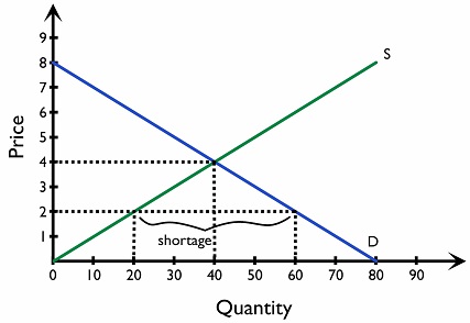
Table 2.7.2.1 summarizes the calculations on impacts of price ceiling which would be required.
Assumption: The available output is bought by consumers with the highest willingness to pay. This gives the consumer surplus shown in the table. Queuing costs, black-market payments and inefficient rationing are excluded; including them can reduce welfare further.
Table 2.7.2.1 Impacts of price ceiling
| Before price ceiling | After price ceiling | |
|---|---|---|
| Price | $4 | $2 |
| Quantity demanded | 40 | 60 |
| Quantity supplied | 40 | 20 |
| Excess demand/shortage | \( 60-20=40\) | |
| Consumer surplus | \(\dfrac{($8-$4)\times 40}{2}=$80\) | \(\dfrac{($8-$6)\times 20}{2}+($6-$2)\times 20=$100\) |
| Producer surplus | \(\dfrac{$4\times 40}{2}=$80\) | \(\dfrac{$2\times 20}{2} = $20\) |
| Consumer expenditure/
Producer revenue |
\($4\times 40=$160\) | \( $2 \times 20 = $40\) |
| Welfare loss | \( \dfrac{($6-$2) \times 20}{2} = $40\) |
Hurricane Katrina reached Category 5 over the Gulf of Mexico, but made landfall in Louisiana on 29 August 2005 as a Category 3 hurricane. It caused severe damage in New Orleans and the surrounding area.
After Hurricane Katrina in August 2005, damaged water supplies and transport links made drinking water difficult to obtain. A shortage of a necessity places particular pressure on low-income households: if its price rises, they may have to reduce spending on other essentials.
A price ceiling is one possible response to such a shortage. However, unless supplies also increase, a price ceiling below equilibrium leaves excess demand; emergency distribution and restoration of water supplies may therefore be needed alongside price controls.
A price floor, also known as a minimum price, refers to the setting of a price higher than the market equilibrium by the government and no seller can sell the goods at a price lower than the minimum price.
The government imposes a price floor for several reasons:
- To protect the sellers and stabilise their income. An example is the agricultural products support that increase and stabilise farmers’ income over the years.
- To prevent deprivation for disadvantaged sellers. The government sets a minimum wage in the labour market so that labour can at least earn a reasonable level of income to maintain their living standard.
Figure 2.7.3 shows the effects of a price floor on the market. An effective price floor has to be set above the equilibrium price \(P_e\). When the price floor of \(P_f\) is imposed, the price is increased from \(P_e\) to \(P_f\). At \(P_f\), the producer is willing and able to supply at \(Q_2\) while the consumer is only willing and able to buy at \(Q_1\). A surplus of \((Q_2-Q_1)\) units exists at the price \(P_f\). The quantity transacted is reduced from \(Q_e\) to \(Q_1\).
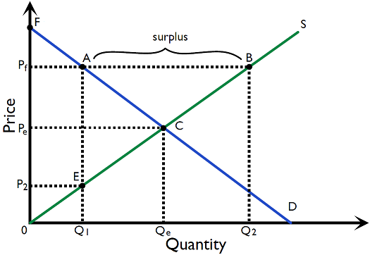
The impact of a price floor
1) Government measures to dispose of the surpluses
At the price \(P_f\), the quantity supplied exceeds the quantity demanded and a surplus occurs. If the government decides to purchase the surplus in order to maintain the price at \(P_f\), the amount spent on government purchase is represented by the area \((ABQ_2Q_1)\). The expense is financed by taxpayers and incurs a cost to society.
2) Effects on producers and consumers
If the government buys all excess supply, producers sell \(Q_2\) units and receive revenue of \(P_f \times Q_2\), represented by \(0P_fBQ_2\). Without government purchases, only \(Q_1\) units are sold and revenue is \(P_f \times Q_1\); whether this exceeds the original revenue depends on the price and quantity changes. Consumers pay a higher price and buy less.
3) Loss of social welfare
The following welfare comparison assumes no government purchases, no externalities, and that the lowest-cost producers supply the units sold. In Figure 2.7.3, initial consumer surplus is \(FP_eC\) and producer surplus is \(0CP_e\). After the price floor, consumer surplus is \(FAP_f\) and producer surplus is \(0EAP_f\). Total surplus falls from \(0FC\) to \(0EAF\), giving a welfare loss of \(ACE\). If the government instead buys the surplus, this comparison no longer applies: government expenditure, the cost of producing the extra units, and any benefit from their eventual use must also be considered.
4) Inefficient resource allocation
Since the government may buy all the surplus of goods, producers have an incentive to overproduce, resulting in inefficient resource allocation.
Calculation of effects from the price floor
Figure 2.7.4 shows the effect of a price floor of $6 on the market.
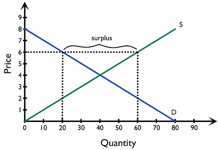
Table 2.7.4.1 summarizes the calculations on impacts of price floor which would be required.
Assumptions: Only the quantity demanded at the price floor is sold, and it is supplied by the lowest-cost producers. The government does not buy the unsold surplus. Government purchasing or a different allocation among producers would change the surplus calculation.
Table 2.7.4.1 Impacts of price floor
| Before price floor | After price floor | |
|---|---|---|
| Price | $4 | $6 |
| Quantity demanded | 40 | 20 |
| Quantity supplied | 40 | 60 |
| Excess supply/surplus | \( 60-20=40\) | |
| Consumer surplus | \(\dfrac{($8-$4)\times 40}{2}=$80\) | \(\dfrac{($8-$6)\times 20}{2}=$20\) |
| Producer surplus | \(\dfrac{$4\times 40}{2}=$80\) | \(\dfrac{($2-$0)\times 20}{2}+($6-$2)\times 20 = $100\) |
| Consumer expenditure/
Producer revenue |
\($4\times 40=$160\) | \( $6 \times 20 = $120\) |
| Welfare loss | \( \dfrac{($6-$2) \times 20}{2} = $40\) |
The Common Agricultural Policy (CAP) is an EU policy launched in 1962 which aims to support farmers, safeguard EU farmers, tackle climate change, and promote jobs in agriculture.
One of the ways that the CAP achieves its aims is through implementing minimum guaranteed prices to European farmers. When the CAP was implemented, the EU guaranteed that it would buy surplus agricultural output to create a buffer stock which could be used when food was more scarce. However, this led to criticism as farmers were incentivised to over-produce, leading to news stories about ‘mountains’ and ‘lakes’ of surplus food and drink which were being left to rot.
Indirect taxes
Indirect taxes are taxes on the expenditure of goods and services. It increases the cost of production and shifts the supply curve to the left. Governments impose indirect taxes for several reasons:
- To finance government expenditure
- To discourage socially undesirable activities, e.g. the government raises the gasoline tax to discourage people driving and hence reducing pollution
- To promote economic growth, e.g. governments impose tariffs to lower the consumption of imported goods as they do not help domestic economic growth
Indirect taxes can be imposed on specific and ad valorem bases.
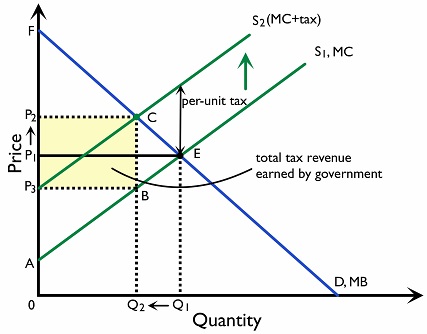
Specific tax/per unit tax means a fixed amount of tax is added onto the goods or services, e.g. a tax of US$100 is imposed on every air ticket. A specific tax raises the cost of production, which reduces supply and shifts the supply curve to the left from \(S_1\) to \(S_2\) in Figure 2.7.5. The vertical distance between the new and old supply curves is the size of the per-unit tax.
Ad valorem tax means a percentage of the total expenditure is taxed, e.g. value-added tax (VAT) where a consumer has to pay an extra 20% of the expenditure in tax.
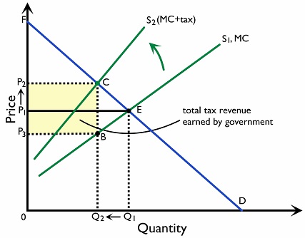
An ad valorem tax has a similar effect with specific tax. It raises the cost of production and shifts the supply curve to the left from \(S_1\) to \(S_2\). However, the shift is not a parallel shift, unlike specific tax. The vertical distance widens at higher prices, as the absolute amount of tax increases when the price of the good is higher. (Figure 2.7.6)
In the UK, one of the main indirect taxes is Value Added Tax (VAT). The standard rate of VAT is 20%; this means that for the majority of goods, consumers pay a tax of 20% when purchasing the good. This tax is included in the price; for example, if a consumer bought a car for £18,000, the price of the car itself would be £15,000, and the VAT on the purchase would be £3,000.
The UK also applies a reduced VAT rate of 5% to certain goods and services, including children’s car seats and domestic energy. Most food and children’s clothes are zero-rated: VAT is charged at 0%. This differs from exemption; for example, qualifying postage stamps are exempt. Zero-rated sales are taxable supplies, allowing the seller to recover eligible input VAT.
Impacts of a specific indirect tax
An imposition of an indirect or ad valorem tax on goods and services will increase the market price level and reduce the quantity transacted of goods and services. Take Figure 2.7.5 as an example: imposition of the indirect tax causes the price to increase from \(P_1\) to \(P_2\), and the quantity transacted to decrease from \(Q_1\) to \(Q_2\).
The imposition of indirect tax has impacts on various stakeholders in the market (Figure 2.7.5):
Consumers: Consumers are worse off because they have to pay a higher price to purchase goods and services. After the imposition of an indirect tax, the total consumer expenditure might increase or decrease depending on the PED. If the PED is inelastic, the total consumer expenditure will increase. If the PED is elastic, the total consumer expenditure will decrease.
Producers: Producers’ revenue decreases. The total revenue producers receive before tax imposed is \((P_1 \times Q_1)\). After the tax is imposed, producers receive a total revenue of \((P_3 \times Q_2)\). Although the market price is \(P_2\), the tax per unit \((P_2 - P_3)\) goes to the government and producers only pocket the amount at \(P_3\). The total revenue for producers decreases and producers are worse off.
Government: The government collects tax revenue equivalent to tax per unit x total after-tax quantity transacted, which is represented by \((P_2 - P_3) \times Q_2\).
Society: A welfare loss of \(CBE\) is incurred after tax is imposed. Before tax, consumer surplus is represented by area \(FEP_1\) and producer surplus is represented by area \(P_1EA\). After tax, consumer surplus becomes \(CFP_2\), while producer surplus becomes \(ABP_3\); the government gains revenue of \(P_2P_3BC\), and the total social surplus is still less than the situation without tax. Now the area of \(CBE\) becomes unattained. Resources are misallocated as there is potential gain not being captured.
Tax incidence and price elasticity of demand and supply
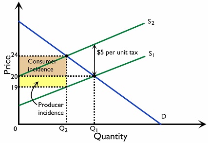
Tax incidence/tax burden refers to the eventual tax payment by a specific party e.g. consumers. For example, a per unit tax of $5 on cigarettes pushes the price up by $4 from $20 to $24, and the after-tax quantity transacted is 10. We say that the tax incidence on the consumer is $4\( \times \)10 = $40 and the tax incidence on the producer is $1\( \times \)10. Consumers have a larger tax incidence. The distribution of tax incidence between producers and consumers is dependent upon the PED and PES.
When demand is less elastic compared to supply, the market price will increase relatively more and consumers pay a larger tax incidence than producers (Figure 2.7.7).
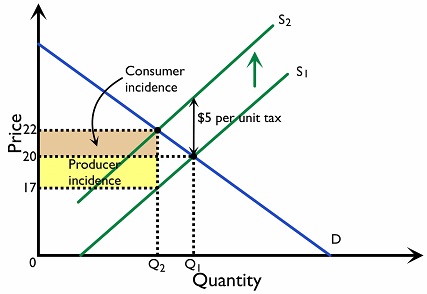
When demand is more elastic compared to supply, the market price will increase relatively less and consumers pay a smaller tax incidence than producers (Figure 2.7.8).
The table below summarises the situations of tax incidences between producers and consumers:
Table 2.7.8.1 Implications of tax incidence on producers and consumers at different levels of PED and PES
|
|
Implications of tax incidence on producers and consumers |
|---|---|
| PES < PED | Producers bear a larger tax incidence |
| PED < PES | Consumers bear a larger tax incidence |
| PES = PED | Tax incidence on producers and consumers are the same |
| PES = 0 | 100% of tax incidence is on producers |
| PED = 0 | 100% of tax incidence is on consumers |
| PES \( \rightarrow \infty \) | 100% of tax incidence is on consumers |
| PED\( \rightarrow \infty \) | 100% of tax incidence is on producers |
Calculations of the effects of a tax on linear demand and supply curves
In Figure 2.7.9, the original demand and supply curves are plotted. When a specific tax of $3 is imposed, the supply curve will shift vertically upward by the amount of tax ($3).
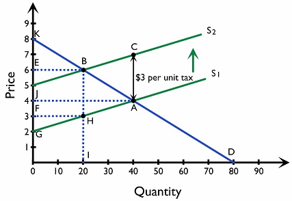
Table 2.7.9.1 summarises the calculations on impacts of taxation which would be required:
| Table 2.7.9.1 Impacts of taxation | ||
|---|---|---|
| P (after tax) | $6 | |
| Q (after tax) | 20 | |
| Incidence on consumers | \( ($6-$4) \times 20 = $40 \) | |
| Incidence on producers | \((\$4-\$3)\times20=\$20\) | |
| Post tax consumer expenditure | Area \(0EBI\) | \( $6 \times 20 = $120\) |
| Post tax producer revenue | Area \(0FHI\) | \( $3 \times 20 = $60\) |
| Government revenue | Area \(FEBH\) | \( $3 \times 20 = $60\) |
| Initial consumer surplus | Area \(KJA\) | \( \dfrac{($8-$4) \times 40 }{2} = $80 \) |
| New consumer surplus | Area \(KEB\) | \( \dfrac{($8-$6) \times 20 }{2} = $20 \) |
| Initial producer surplus | Area \(AJG\) | \( \dfrac{($4-$2) \times 40 }{2} = $40 \) |
| New producer surplus | Area \(FGH\) | \( \dfrac{($3-$2) \times 20 }{2} = $10 \) |
| Initial total social surplus | Area \(AKG\) | \( $80 + $40 = $120 \) |
| New total social surplus | Area \(KBHG\) | \( $20 + $10 + $60 = $90 \) |
| Welfare loss | Area \(ABH\) | \( $120 - $90 = $30 \) |
To facilitate calculations, it is best to draw the diagrams to visualise the effects of the impacts of tax on producers and consumers.
Subsidies
Subsidies are grants provided by the government to firms aiming at lowering production costs and increasing output. Governments impose subsidies for several reasons:
- To promote exports by lowering the price of goods so they are more competitive in the foreign markets.
- To encourage socially beneficial activities, e.g. the government provides subsidies to community centres to hold activities for citizens.
- To encourage consumption on merit goods, e.g. the government grants subsidies on education and healthcare services.
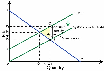
In Figure 2.7.10, when the government provides a per-unit subsidy, it lowers the production cost and increases the supply from \(S_1\) to \(S_2\). The vertical distance between \(S_1\) and \(S_2\) is the per unit subsidy provided.
Housing subsidies aim to support access to housing and may also encourage construction. In the US, housing support includes tax relief, such as the mortgage interest deduction on federal income tax, which reduces taxable income rather than the contractual mortgage interest rate. Down-payment assistance is another form of support, but eligibility, funding and repayment conditions depend on the particular programme. Source: GAO historical housing-assistance analysis; not support for the $15bn claim
Impact of subsidies
Imposing a subsidy on goods and services will decrease the market price level and increase the quantity transacted of goods and services. Take Figure 2.7.10 as an example: an imposition of subsidy causes the price to decrease from \(P_1\) to \(P_2\), and the quantity transacted to increase from \(Q_1\) to \(Q_2\).
Imposition of subsidy has impacts on various stakeholders in the market (Figure 2.7.10):
Consumers: Consumers are better off because they pay a lower price to purchase goods and services. After the imposition of a subsidy, the total consumer expenditure might increase or decrease depending on the PED. If the PED is inelastic, the total consumer expenditure will decrease. If the PED is elastic, the total consumer expenditure will increase.
Producers: Producers’ revenue increases. The total revenue producers receive before subsidy imposed is \((P_1 \times Q_1\)). After a subsidy is imposed, producers receive a total revenue of \((P3 \times Q_2)\). Although the market price is \(P_2\), the per unit subsidy \((P_3 - P_2)\) goes to the producer and the producers pocket the amount at \(P_3\). The total revenue of producers increases and producers are better off.
Government: The government spends subsidy expenditure equivalent to the subsidy per unit x total after-subsidy quantity transacted, which is represented by \((P_3-P_2) \times Q_2\).
Society: In Figure 2.7.10, initial consumer surplus is \(FAP_1\) and producer surplus is \(AEP_1\). After the subsidy, consumer surplus is \(FBP_2\) and producer surplus is \(ECP_3\). The gains are \(P_1P_2BA\) and \(P_1P_3CA\), respectively. However, government expenditure is \(P_2P_3CB\). With no externalities, social surplus is consumer surplus plus producer surplus minus government expenditure. It falls by triangle \(ABC\), because the cost of the extra output exceeds its benefit to consumers. A rise in consumer and producer surplus alone is therefore not a rise in net social welfare.
Calculations of the effects of subsidy on linear demand and supply curves
In Figure 2.7.11, the original demand curve and supply curve is plotted. When a per-unit subsidy is granted, the supply curve will shift vertically towards the right by the amount of subsidy.
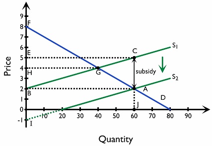
Table 2.7.11.1 summarises the calculations on impacts of subsidies which would be required:
| Table 2.7.11.1 Impacts of subsidies | ||
|---|---|---|
| P (after subsidy) | $2 | |
| Q (after subsidy) | 60 | |
| Post-subsidy consumer expenditure | Area \(0BAJ\) | \( $2 \times 60 = $120 \) |
| Post-subsidy producer revenue | Area \(0ECJ\) | \( $5 \times 60 = $300 \) |
| Government subsidy expenditure | Area \(BECA\) | \( $3 \times 60 = $180 \)
|
| Initial consumer surplus | Area \(FGH\) | \( \dfrac{($8 - $4) \times 40 }{2} = $80 \)
|
| New consumer surplus | Area \(BFA\) | \( \dfrac{($8 - $2) \times 60 }{2} = $180 \) |
| Initial producer surplus | Area \(BHG\) | \( \dfrac{($4 - $2) \times 40 }{2} = $40 \)
|
| New producer surplus | Area \(BEC\) | \( \dfrac{($5 - $2) \times 60 }{2} = $90 \) |
| Initial total social surplus | Area \(BFG\) | \( $80 + $40 = $120 \) |
| New consumer surplus plus producer surplus (before subsidy cost) | Area \(IFA\) | \( $180 + $90 = $270 \) |
| Increase in consumer surplus plus producer surplus | \( $270 - $120 = $150 \) | |
| Welfare loss | Area \(AGC\) | \( $180 - $150 = $30 \) |
The subsidy raises consumer surplus plus producer surplus from $120 to $270, a gain of $150. However, the government spends $180. Net social surplus after the subsidy is therefore $270 − $180 = $90, compared with $120 initially. The welfare loss is $120 − $90 = $30. This example assumes no external benefits from the additional output.
Direct provision of services
Merit goods are goods considered to be beneficial to people that are underprovided by the market and therefore underconsumed, resulting in positive externality from consumption. e.g. vegetables. Consumers may consume insufficiently because they either underestimate the potential benefits or choose to ignore the potential benefits. This means that demand for the good is lower than would be optimal for society.
Governments try to increase the consumption of merit goods. One way to do so is through direct provision; for example, the government might choose to directly provide healthcare to the consumer because it believes that the benefits of healthcare are so important.
However, direct provision may be costly and involve an opportunity cost; for example, if the government chooses to increase its spending on healthcare, it will have to decrease its spending elsewhere. The government may also not be best placed to provide certain goods, for example vocational training.
An example of the direct provision of services by the government is the UK National Health Service (NHS), which has been publicly funded since it was founded in 1948. The NHS is committed to providing comprehensive, universal healthcare which is free at the point of delivery.
There are significant benefits associated with the direct provision of healthcare through the NHS; for example, the NHS has significant market power when purchasing medication, meaning that it can influence the global price and keep prices lower for consumers. The NHS also ensures that all UK residents can access healthcare, meaning that standards of living are significantly higher than they would be under a private healthcare system, where some individuals would be priced out of healthcare.
However, in recent years, public satisfaction in the NHS has fallen. Funding constraints are one possible influence, but this does not establish a single cause of changing satisfaction. Health spending grew more slowly in real terms during 2010–2014, while social-care spending fell. For example, a study of OECD data found that the NHS is significantly under-resourced compared to other developed nations, with among the lowest number of doctors, nurses, and hospital beds per capita. In its 2019 report, the Institute for Public Policy Research estimated that over 130,000 deaths could have been prevented if earlier improvements in preventable mortality had continued. This is a comparison with an extrapolated trend, not a count of deaths proved to have been caused solely by NHS funding cuts. That said, the NHS succeeds in protecting people from heavy financial costs when they are unwell, and has waiting times and efficiency rates comparable to other developed countries.
Command and control regulation and legislation
Demerit goods are goods considered to be harmful to people that are overprovided by the market and therefore overconsumed, resulting in negative externalities from consumption. e.g. cigarettes, alcohol etc. Consumers are either unaware of the harm or choose to ignore the risk. The demand for demerit goods is therefore higher than would be optimal for society.
The government might choose to reduce the demand of demerit goods by passing legislation which alters consumers’ behaviour. For example, the government might make it illegal to smoke in public places or set age restrictions on purchasing cigarettes.
Such regulation might be harmful to the producers of the product. This might lead to the producers lobbying the government to prevent it from bringing in new legislation. Regulation might also be difficult to enforce; this will require the government allocating resources to ensure that consumers comply with regulation.
An example of command and control legislation used to curb demand for demerit goods is the smoking ban in England which came into force in 2007. This legislation made it illegal to smoke in all public enclosed or substantially enclosed areas and workplaces, including public transport. This meant that individuals looking to smoke have to do so outdoors; all indoor smoking areas, such as smoking rooms, were no longer permitted.
According to the BBC, the imposition of the smoking ban has correlated with a decrease in the proportion of the population who smoke, as shown in the graph below.
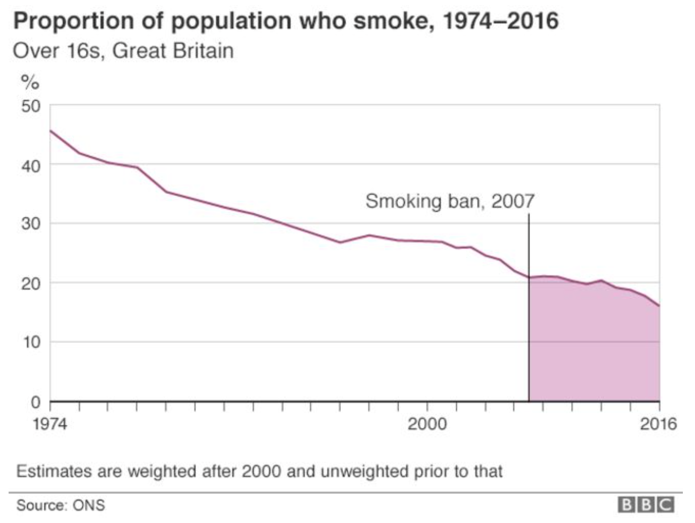
At the same time, the BBC also reported that the numbers of young people taking up smoking have halved since the introduction of the ban, and there was a 23% increase in the number of existing smokers who attempted to quit using NHS stop-smoking services following the imposition of the ban, due to its effectiveness regarding raising the awareness of the risks of second-hand smoke.
The ban on smoking in public places was therefore effective in decreasing demand for a demerit good, and in mitigating the harmful effects of that demerit good on society.
Consumer nudges
Consumers do not always have perfect information, and do not always make rational choices. Governments can use ‘consumer nudges’ to encourage consumers to reduce their consumption voluntarily.
For example, cigarette manufacturers used to use innovative package design to advertise to consumers. Many governments have therefore put in place laws which require cigarette packs to be a plain dull colour with graphic images showing the dangers of smoking in order to ‘nudge’ consumers not to smoke. Consumers still have their freedom of choice, but are nudged to choose differently.
However, this also has the impact of lowering the profits of firms which produce demerit goods. For example, cigarette manufacturers have critiqued this government legislation on the grounds that it removes their freedom to pursue profits.