2.8 Market failure - externalities and common pool or common access resources
Market failure refers to the situation where the price mechanism cannot achieve allocative efficiency. Under market failure, resources are either over-allocated (in which case there is an overprovision of a good), or under-allocated (in which case there is an underprovision of a good) from society’s point of view. Externalities mean the spillover effect on a third party when a good or service is produced or consumed.
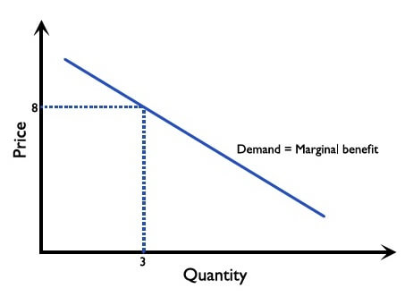
When a good is consumed, a certain level of benefit is derived from the good. Marginal benefit (MB) is the extra benefit that is gained from the consumption of one extra unit. The MB curve is an analogous demand curve: the demand curve shows the consumer’s maximum willingness and ability to pay for each quantity of the good at every price level. The price at each quantity is in fact the MB the consumer receives. For instance, in Figure 2.8.1, the maximum price the consumer is willing and able to pay for the 3rd unit of the good is $8. The MB derived from the 3rd unit of good is therefore equivalent to $8. If the MB is higher, the consumer would be willing to pay more. If the MB is lower, the consumer would be willing to pay less.
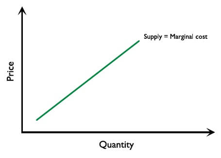
Likewise, when a good is produced, resources are used, and there is a corresponding cost of production. Marginal cost (MC) shows the extra cost needed to produce one extra unit of the good, and the MC curve is an analogous supply curve. (Figure 2.8.2)
Private cost refers to the cost incurred by producers in production e.g. electricity, wage, rent, raw materials etc. External cost refers to the spillover effect on a third party who is not involved in production e.g. pollution. As society includes everyone, social cost can be shown by the equation:
Social cost = Private cost + External cost
When considering marginal social cost (MSC), which is the additional cost to society from an additional unit of production, the equation becomes:
Marginal social cost (MSC) = Marginal private cost (MPC) + Marginal external cost (MEC)
Private benefit means the benefit incurred by consumers in consumption e.g. better education gives better career prospects to students (who are consumers of education). External benefit means the spillover effect on a third party not involved in consumption e.g. higher productivity in society due to better education. As society includes everyone, social benefit can be shown by the equation:
Social benefit = Private benefit + External benefit
When considering the marginal social benefit (MSB), which is the additional benefit to society from additional unit of consumption, the equation becomes:
Marginal social benefit (MSB) = Marginal private benefit (MPB) + Marginal external benefit (MEB)
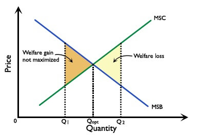
Socially optimal output is at the point where Marginal Social Benefit (MSB) equals Marginal Social Cost (MSC).
Allocative efficiency
Social allocative efficiency is where the marginal social benefit (MSB) = marginal social cost (MSC). The social optimal level of production/consumption has to be at \(Q_{opt}\). It is because that at \(Q_1\), producing an additional unit incurs a higher marginal social benefit than the marginal social cost to society (MSB>MSC), therefore welfare gain for society has not been maximised. At \(Q_2\), producing additional units incurs a higher marginal social cost than the marginal social benefit to society (MSC>MSB). Therefore, welfare loss is incurred on society.
However, as consumers and producers are interested in maximising private welfare, not social welfare, only private costs and benefits are considered when consumers and producers make decisions. Private market equilibrium is where the marginal private benefit (MPB) = marginal private cost (MPC). Externalities shall occur when:
Social optimal quantity (Qsocial) might not be equal to private optimal quantity (Qprivate)
Qsocial > Qprivate , there is underprovision/underconsumption
Qsocial < Qprivate , there is overprovision/overconsumption
Positive externality of production
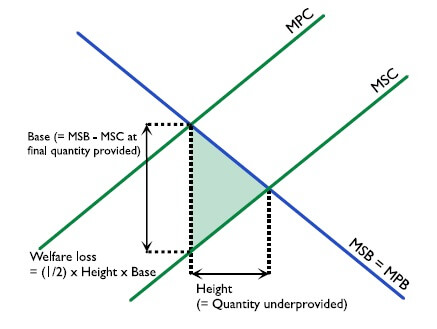
Positive externality of production means that production creates positive effects on a third party. An example is forestry. With more trees planted, people can enjoy cleaner air. When there are positive production externalities, the MSC is lower than the MPC at any given quantity, and is drawn to the right of the MPC, as shown in Figure 2.8.4.
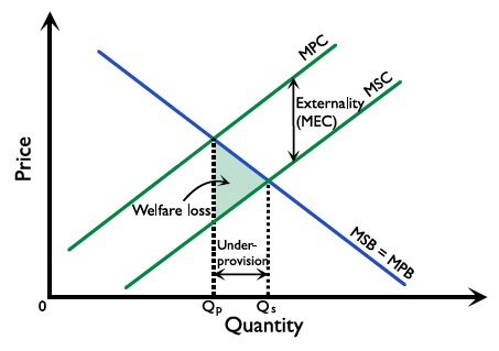
The social optimal quantity is at \(Q_s\), where MSC = MSB. The amount of the good produced in this market is the private market equilibrium quantity \(Q_p\) where MPC = MPB. \(Q_p\) is smaller than the social optimal quantity \(Q_s\), and there
is an underprovision of the good by \((Q_s - Q_p)\).
For each unit produced below \(Q_s\), MSB is greater than the MSC (i.e. to society, production of the good generates more extra benefit than extra cost), and society would be better off if more are produced. Summing up the net benefit of non-production
per unit (MSB \( - \) MSC) over each unit produced below the social optimal quantity \(Q_s\) makes the size of welfare loss/potential welfare gain, which is equivalent to the shaded area in Figure 1.4.7.
When discussing production, only marginal social and private cost curves differ. On the benefit side, it is assumed that MSB = MPB.
Calculation of potential welfare gain/ welfare loss associated with positive externality of production
The calculation of welfare loss makes use of the formula calculating the area of the triangle (\(\frac{1}{2}\) x base x height). The height of the triangle is equivalent to the quantity underprovided, or \((Q_s - Q_p)\). The base is the net benefit per unit (MSB \( - \) MSC) that can be gained from further production, and is at the final quantity provided under a private equilibrium \((Q_p)\). Multiplying the base and height and dividing the result by 2 gives the size of welfare loss in monetary terms.
Positive externality of consumption
Positive externality of consumption means that consumption creates positive effects on a third party. An example would be education. The student (consumer) benefits from education e.g. better career prospects, firms in society (third party) benefit from a more productive labour force.
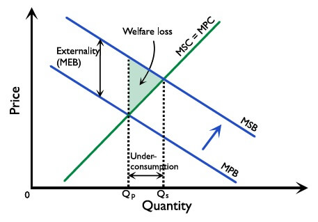
When there are positive externalities of consumption, the MSB is higher than the MPB at any quantity, and the MSB is thus drawn to the right of the MPB, as shown in Figure 2.8.6. The vertical difference between the MSB and MPB is the extent of the marginal external benefit (MEB) at any quantity.
The social optimal quantity is at \(Q_s\), where MSC = MSB. The amount of the good produced in this market is the private market equilibrium quantity \(Q_p\) where MPC = MPB. \(Q_p\) is smaller than the social optimal quantity \(Q_s\), and there is underconsumption of the good by \((Q_s – Q_p)\).
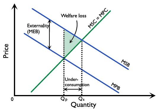
For each unit consumed below \(Q_s\), the MSB is greater than the MSC (i.e. to society, continual production of the good would generate more extra benefit than extra cost), and society would be on the whole better off if more is consumed. Summing up the potential net gain (MSB – MSC) over each unit consumed below the social optimal quantity \(Q_s\) gives the size of welfare loss/potential welfare gain, equivalent to the shaded area in Figure 2.8.6.
Merit goods
Merit goods are goods considered to be beneficial to people that are underprovided by the market and therefore underconsumed, resulting in positive externality from consumption. e.g. vaccination, vegetables etc.
Students often confuse the terms merit good and positive externality. Merit good refers to a good that has positive externalities; positive externality refers to the effect incurred on a third party.
Negative externality of production
Negative externality of production means that production creates adverse effects on a third party e.g. pollution. An example would be a factory that produces garments and emits pollutants into the river, affecting the health of the villagers (third party) living downstream.
When there are negative production externalities, the MSC is greater than the MPC at any given quantity, and the MSC is thus drawn on the left of the MPC, as shown in Figure 2.8.7. The vertical distance between the MSC and MPC is the extent of the marginal external cost (MEC) at any given quantity.
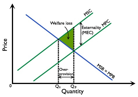
The social optimal quantity is at \(Q_s\) where MSC = MSB. However, the amount of goods produced in this market is at \(Q_p\). \(Q_p\) corresponds to the private market equilibrium, where MPC = MPB. However, \(Q_p\) is greater than the social optimal
quantity, \(Q_s\), and there is an overprovision of the good by \((Q_p - Q_s)\). For each unit produced beyond \(Q_s\), the MSC is greater than the MSB (to society, the production of an extra unit generates more extra cost than extra benefit),
and society would be better off if the quantity \((Q_p - Q_s)\) is not produced. Summing up the net loss incurred from every unit of overproduction (MSC\( - \)MSB) over all quantities produced beyond the social optimal quantity \((Q_p - Q_s)\)
gives the area of welfare loss equal to the shaded area in Figure 2.8.7.
Calculation of welfare loss associated with negative production externality
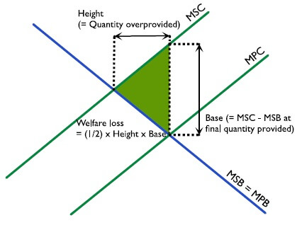
Consider the formula calculating the area of triangle (\( \frac{1}{2} \)x base x height). Figure 2.8.8 shows that the height of the triangle is equivalent to the quantity overprovided, or \((Q_p - Q_s)\). The base is the net loss (MSC\( - \)MSB) at the final quantity provided \((Q_p)\). Multiplying the base and height and dividing the result by 2 gives the size of welfare loss in monetary terms.
Negative externality of consumption
Negative externality of consumption means that consumption creates adverse effects on a third party. An example would be smoking; where when one person smokes (consumer) it causes another
person (third party) to suffer from second hand smoke.
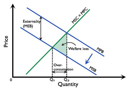
When there are negative externalities of consumption, MSB is lower than MPB at any quantity, and MSB is thus drawn to the left of MPB, as shown in Figure 2.8.9. The vertical difference between MSB and MPB is the (negative) marginal external benefit
(MEB) at any given quantity.
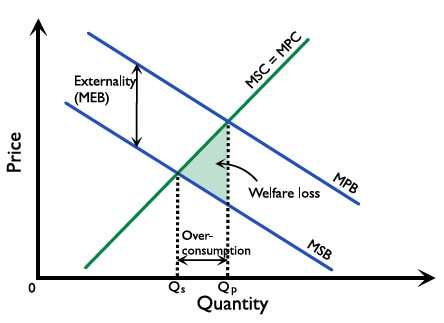
The social optimal quantity is at \(Q_s\), where MSC = MSB. The amount of the good produced in this market is the private market equilibrium quantity \(Q_p\) where MPC = MPB. \(Q_p\) is greater than the social optimal quantity \(Q_s\), and there
is overconsumption of the good by \((Q_p – Q_s)\).
For every unit consumed beyond \(Q_s\), the MSC is greater than the MSB (i.e. to society, consumption of the good generates more extra cost than extra benefit), and society would be better off if the excess quantity of \((Q_p - Q_s)\)
is not consumed. Summing up the net loss incurred per unit consumed (MSC \( - \) MSB) over each unit consumed beyond the social optimal quantity \((Q_s)\) gives the area of welfare loss, equivalent to the shaded area in Figure 2.8.9.
Demerit goods
Demerit goods are goods considered to be harmful to people that are overprovided by the market and therefore overconsumed, resulting in negative externalities from consumption. e.g. cigarettes, alcohol etc.
Students often confuse between the terms demerit good and negative externality. Demerit good refers to a good that has negative externalities; negative externality refers to the effect incurred on a third party.
Common pool resources
Common pool resources are resources like fishing grounds and pastures which exhibit the following characteristics:
- They are non-excludable: it is not possible to prevent individuals who have not paid for a good from using it.
- They are rivalrous: the consumption of the good by one individual does prevent simultaneous consumption by another individual.
The tragedy of the commons refers to a situation where the effect of all rational producers acting in their own self-interest results in a fall in social welfare. A common example of this is an area of pasture which is open to all cattle herders; each cattle herder acts rationally and wants to maximise their own self-interest, so grazes as much cattle as possible on the field. However, when all cattle herders think the same way, there is over-grazing on the field and the resource is destroyed. Therefore, producers, seeking to maximise their own well-being, impose external costs on others.
Even if some of the herders were to realise what was happening and change their behaviour, this would result in the free rider problem: those who did not change their behaviour would benefit from those who do.
Examples of common pool resources that pose a threat to sustainability
1) Fossil fuels & atmospheric air
There is no ownership of atmospheric air. It has a finite capacity and limited rate of dissipation of greenhouse gases, and can therefore be considered as an example of a common access resource. The use of fossil fuels generates greenhouse gases. When an excessive amount of greenhouse gases are released into the atmosphere, the atmosphere cannot dissipate them quickly enough, leading to global warming. Global warming is a symptom of unsustainable development. Producers of fossil fuels bear the private costs of production, e.g. rent, wage, raw materials etc. The third party bears the external cost e.g. pollution, global warming etc. Therefore, the use of fossil fuels generates negative externality of production. This effect can be illustrated using a negative externality diagram, as shown in Figure 2.8.7 for use of fossil fuels in production.
2) Poverty and overexploitation of land for agriculture
Agriculture is the main provider of employment (and food) in developing countries, especially among the rural poor. Increased population growth and poverty in developing countries have driven many rural farmers to exploit more land using intensive farming methods, even in fragile environments. While this can maximise farm yields in the short-term, it is unsustainable because the soil cannot recover nutrients quickly enough, leading to soil degradation in the long term. As soil degradation can be viewed as an adverse spillover effect on a third party, e.g. forgoing the use of soil by a third party, over exploitation of land can be seen as a type of negative externality of production.
Government intervention in response to externalities and common pool resources
Indirect (Pigouvian) taxes
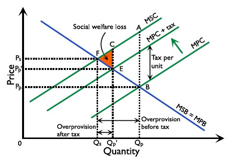
The government can impose a Pigouvian tax to reduce the level of output from negative externalities. Referring to Figure 2.8.10, when an indirect tax is being imposed on production that creates negative externalities, the cost of production increases and supply decreases. This shifts the MPC curve from MPC to MPC + tax. The quantity of output produced decreases from \(Q_p\) to \(Q_p’\), which is closer to the social optimal level \(Q_s\). The area of welfare loss decreases from \(ABF\) to \(CEF\). If the indirect tax imposed is equivalent to the external cost generated, the private market output level can be restored to the social optimal level. Indirect taxes reduce the problem of overproduction.
Referring to Figure 2.8.11, when an indirect tax is being imposed on consumption that creates negative externalities e.g. cigarettes, alcohol etc, the cost of production increases and supply decreases. This shifts the MPC to MPC + tax. The private market consumes at MPC + tax = MPB. Consumption level decreases from \(Q_p\) to \(Q_p’\), which is closer to the social optimal level \(Q_s\). Indirect taxes reduce the problem of overconsumption.
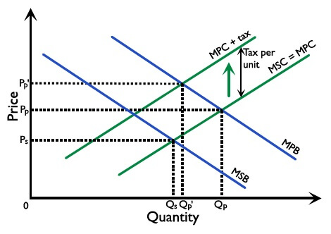
The effectiveness of indirect taxes depends on the elasticity of demand and supply; if the demand is more inelastic than the supply, the government will need to impose a higher per unit tax to reduce overprovision/overconsumption. At times the MSB (or MSC) and its equivalent monetary value is hard to determine, for instance in the case of taxes for cigarettes.
The use of indirect taxes would place large informational demands on the government. The government needs to know the MSC and MPC (negative externality of production) or the MSB and MPB (negative externality of consumption) of the private market to set the correct level of taxes, but it is often difficult and costly to obtain the information.
Indirect taxes are also regressive; that is, they impact people who have lower incomes more than they impact people who have higher incomes, as each group pays the same amount of tax but this takes up a larger proportion of income for lower income people.
Governments often use indirect taxes to reduce consumption of demerit goods such as cigarettes. A US statistical table reported a weighted average cigarette excise-tax share of 44.3% of the retail price as of 1 November 2016. The calculation included federal and state cigarette taxes, with specified local-tax adjustments, and excluded sales tax. Source: NC Department of Revenue, 2017 Statistical Abstract, Table 7
A 2009 California tobacco-control report summarised earlier research suggesting that a 10% rise in cigarette prices was associated with nearly a 7% reduction in youth smoking prevalence. This is a historical estimate of a relative percentage change in the proportion who smoke, not a seven-percentage-point fall or a response that must occur in every market. However, cigarette taxation can place a substantial burden on low-income people who continue to smoke. Using 2010–2011 survey data, a 2012 study found that lower-income smokers in New York spent 23.6% of household income on cigarettes, compared with 2.2% for higher-income New York smokers. Those expenditure figures do not establish that higher taxes failed to encourage quitting. Source: California strategy report (2009), government-hosted copy
Carbon taxes
A carbon tax is a tax imposed when fossil fuels are burned; this is a way to make producers of carbon emissions pay for the external costs that are not included in the market price.
A carbon tax aims to force the producer to pay the full cost of producing the product. To completely eliminate the negative externality created when carbon is emitted, the government would have to be able to calculate the external costs and set the tax to reflect those costs; however, in practice a carbon tax may not completely eliminate the welfare loss.
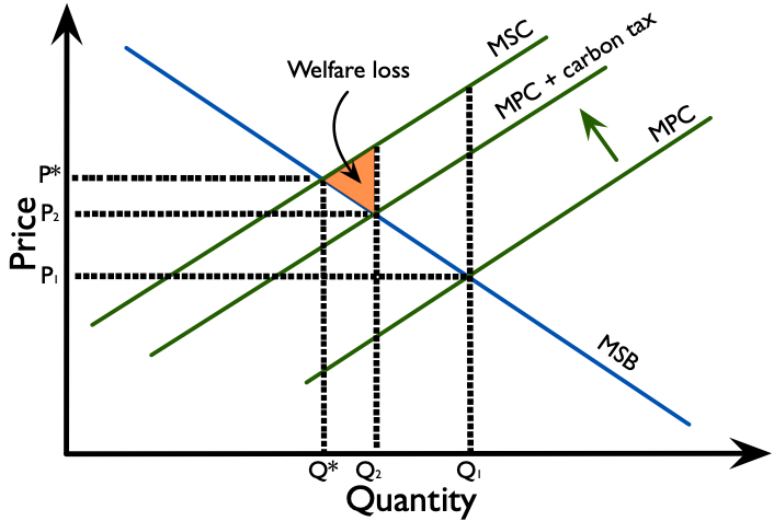
In Figure 2.8.12, the market price \(P_1\) does not reflect the external costs of producing carbon emissions. Adding a $10 tax to production shifts the supply curve up closer to the Marginal Social Cost curve, and shifts the market price to \(P_2\), which is closer to the market optimum, \(P*\).
Carbon taxes are beneficial because they incentivise producers to invest in new technologies that will reduce their emissions. They may also have an incentive to reduce their electricity consumption by switching to more energy-efficient appliances. The tax will generate revenue for the government which can be used to subsidize renewable energies to make them more affordable for consumers.
In 2020, British Columbia, Canada, had a carbon tax rate of $40 per tonne of CO2 equivalent emissions. This is calculated to be consistent with estimates of the social cost of carbon, which is the economic value of avoided climate change damages for current and future generations as a result of reducing greenhouse gas emissions.
Research has shown that the carbon tax in British Columbia reduced the consumption of gasoline and natural gas, and therefore led to a reduction in overall emissions of CO2. For example, per capita emissions decreased by 12.9% in 2008-2013, three and a half times more than the per capita decline in the rest of Canada. The tax also incentivised people to buy fuel-efficient vehicles. In 2012-13, this carbon tax raised around $1,120 million in revenue. Under the revenue-neutral arrangements then in place, revenue was returned through tax reductions and credits. It was not a fund earmarked for environmental projects.
Policy date: This is a historical case about the carbon tax operating in 2008–2020. British Columbia ended its consumer carbon tax on 1 April 2025. That change should not be confused with ending every form of industrial carbon pricing. British Columbia: 2025 change
Legislation and regulation
The government might choose to combat positive and negative externalities by passing legislation which alters consumers’ behaviour.
In the case of a positive externality, the government might pass a law which, for example, insists that citizens have vaccinations against certain diseases. However, this may be unpopular unless the government provides the service free of charge. People may also resent the imposition on their civil liberties.
The extent to which the government will intervene depends on the extent of the external benefits. These are difficult to measure. It may also be the case that the private sector is better placed to ensure efficiency in production in some sectors, so government provision leads to inefficiency.
In the case of a negative externality, for example, the government might make it illegal to smoke in public places or set age restrictions on purchasing cigarettes.
Such regulation might reduce the demand for demerit goods, and therefore shift the demand curve inwards and reduce the externality, as shown in Figure 2.8.13.
Such regulation might be harmful to the producers of the product. This might lead to the producers lobbying the government to prevent it from bringing in new legislation. Regulation might also be difficult to enforce; this will require the government allocating resources to ensure that consumers comply with regulation.
England introduced a 5p charge on single-use plastic carrier bags at large retailers on 5 October 2015. The charge aimed to reduce the number of bags supplied, encourage reuse and reduce litter. It was not a tax paid to the government. From 21 May 2021, England increased the charge to 10p and extended it to all retailers. The results below concern the earlier policy.
Conventional plastic bags are generally made from fossil-fuel feedstocks, and their production and disposal can impose environmental costs. They persist in the environment; breakdown depends on the material and surrounding conditions, and fragmentation into microplastics is not complete biodegradation. Discarded plastic can harm marine wildlife through ingestion and entanglement. Sources: UNEP/MAP communication (2014); UNEP plastic-pollution communication (2019)
The plastic bag charge has had a significant impact on the use of plastic bags in England. For example, in 2013, major supermarkets in England gave out over 7.4 billion plastic bags. In 2018, it was found that the charge has reduced plastic bag sales in major supermarkets by 86%.
Education - awareness creation
Consumers do not necessarily have perfect information about the damage that demerit goods might cause them or the benefits of merit goods. Governments could therefore increase the information available to consumers through education or an awareness campaign in order to influence demand for demerit and merit goods.
Reducing demand for demerit goods would shift the MPB curve to the left, reducing the externality. Increasing demand for merit goods would shift the MPB curve to the right, reducing the welfare loss from under-consumption.
However, education and awareness campaigns may be costly, and may also be ineffective. Behavioural economics argues that it may be the case that consumers are aware of potential risks but convince themselves that they will not be affected.
‘The Real Cost’ is a US Food and Drugs Administration (FDA) campaign which aims to educate teenagers about the effects of cigarette smoking, including e-cigarettes.
In the US in 2017, 2.1 million middle- and high-school students reported that they were using e-cigarettes; this rate increased rapidly in the following years. The FDA therefore aimed to address the mentality that e-cigarettes were ‘safe’ or ‘cost-free’ by educating young people about the fact that e-cigarettes also carry a risk of addiction and other health consequences. The campaign used television ads, online video ads, a website, social media, and posters in high schools across the US.
The FDA estimates that its campaign has stopped around 587,000 young people across the US from starting to smoke between the launch of the campaign in February 2014 to November 2016. It further estimated that stopping this number of young people from smoking would save more than $53 billion for society by reducing smoking-related costs like early loss of life, medical care, lost wages, lower productivity, and increased rates of disability.
Tradable permits
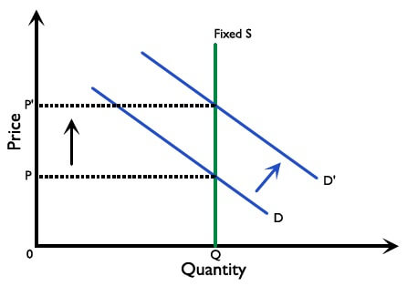
Negative production externalities (especially those related to pollution) can be corrected by the use of tradable permits. Tradable permit means each firm (or individual) that owns permits has the right to emit a quantity of pollutants determined by the permits. These permits can be bought and sold. The total supply of permits is fixed by the government. The price of the permit is determined by the level of demand and supply in the market. When demand increases as in Figure 2.8.16, price increases. By controlling Q, the government is able to control the maximum amount of pollutant released. One of the largest tradable permit systems is the European Union Emissions Trading System for carbon dioxide emissions.
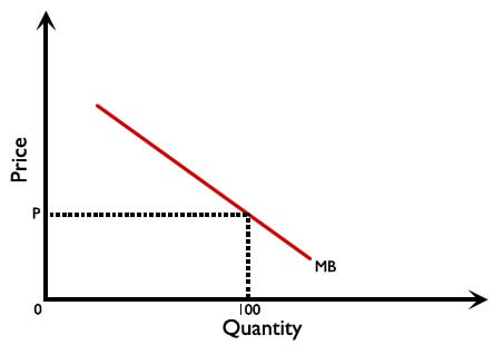
Holders of permits can either choose to use the permit, or sell it on permit markets. Use of the permit entails an opportunity cost equivalent to the income foregone by not selling the permit. A firm would use permits only up to a point where marginal benefit of the permit is equal to the market price (MB = P). If MB is less than P, the firm would be better off selling the permit.
Firms that need extra permits can, in turn, buy them. They would also buy permits only up to a point where the marginal benefit of a permit is equal to the market price (MB = P). For example, at price P in Figure 2.8.16 and 2.8.17, firm A will buy up to 100 tons of CO2 permits. If MB falls below P, the firm will not buy the permit. A tradable permit market is efficient: permits are distributed in such a way where it is not possible to increase the overall social benefit by redistributing a permit to another firm that can generate higher MB. Firms are also incentivised to reduce emissions, because there is a cost for using permits (income foregone, or expenses used to buy permits).
However, there are costs in establishing and managing permit markets. Insufficient demand for permits (because of overallocation or new technology reducing emissions) can lead to a collapse of market prices. Speculation in the permit markets can also cause high price volatility.
The EU Emissions Trading System (EU ETS) launched in 2005. It is one of the world’s largest emissions-trading systems. The original case reports an estimated reduction of more than 1 billion tonnes of CO₂ between 2008 and 2016, equivalent to 3.8% of EU-wide emissions. Its earlier framework targeted a 43% reduction in covered-sector emissions by 2030 relative to 2005. The revised framework raises that 2030 target to 62%.
The ETS aims to reduce climate change emissions in a cost-effective way. In the historical coverage described around 2020, it operated in all the EU countries plus Iceland, Liechtenstein and Norway, and limited emissions from over 11,000 installations using energy, and the airlines operating between those countries, meaning that it covered around 45% of the EU’s greenhouse gas emissions.
The ETS is a cap-and-trade scheme. That means that a ‘cap’ is set on the total amount of greenhouse gas emissions that can be emitted by the installations that are covered by the system, with this cap being reduced over time so that total emissions fall. Within the cap, the companies receive or buy emissions allowances, which they can trade between themselves as required. If a company emits more than it has permits for, it is heavily fined.
International agreements
International agreements are vital for reducing the over-consumption of common pool resources such as the environment and fisheries globally. Although individual governments have important roles to play, the global nature of the problem, and the fact that ‘the environment’ is not limited to each country, means that international agreements are necessary.
One example of an international agreement on climate change is the United Nations Framework Convention on Climate Change (UNFCCC) which provides a framework for negotiations and agreements. The Intergovernmental Panel on Climate Change (IPCC) was set up in 1988 to provide policymakers with assessments of the scientific basis of climate change and assessments of its impacts and risks.
The Kyoto Protocol was created under the UNFCCC in 1997, with the aim of cutting global emissions of greenhouse cases. It had some success in reducing emissions in signatory countries but did not reduce global emissions.
The Paris Agreement in 2015 intended to keep the global temperature rise resulting from climate change to below 2 degrees Celsius. It also recognised the interrelationship between human rights and climate change, as global warming threatens rights like the access to shelter, particularly in developing countries.
However, these are not perfect solutions. Not all countries are committed to the process, and at least one has said that it will remove itself from the agreement because it is worried that the requirements will damage its economic growth. Governments are short-sighted, and more concerned about high rates of economic growth and political popularity rather than the long-term issue of climate change which, they think, will only affect future governments.
There are also concerns about supporting developing countries, and about monitoring and enforcement to ensure that countries meet their commitments.
Collective self-governance
Common suggestions for overcoming the tragedy of the commons are government control and private ownership. Another possible solution, proposed by Elinor Ostrom, is for individuals and communities to work together without regulation to develop rules to manage their shared resources in a sustainable manner.
This is beneficial as there is no ‘one size fits all’ approach to managing a particular resource, and the communities who benefit from the resources have the greatest incentive to maintain them well and ensure their sustainability. They are also more likely to implement, monitor, and enforce the rules that they themselves have set.
A historical example of collective self-governance in response to the depletion of a common access resource is the Japanese sandeel stock in Ise Bay, which serves fisheries in the Aichi and Mie Prefectures. Given the nature of this resource, harvesting tends to be concentrated in the two or three weeks immediately after the fishing season opens; there is therefore a risk of over-harvesting.
Over-fishing led to poor harvests between 1978 and 1982. In response to this, sandeel fishers implemented resource management measures including setting the opening and closing dates of fisheries, and establishing protected areas. These measures were designed and implemented through collaboration between fishers and local researchers.
The case illustrates cooperation between fishers and researchers, but it should not be read as evidence of permanent stock recovery. Aichi’s fisheries report of 17 March 2026 recorded that the fishery would not open. Later closures do not, by themselves, establish the cause of stock depletion.
Subsidies
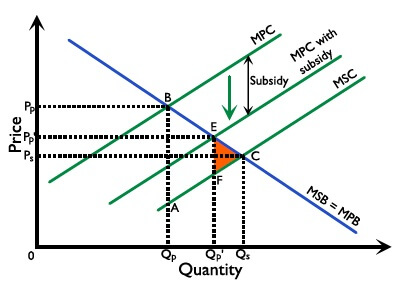
The government can impose a subsidy to increase the level of output. Referring to Figure 2.8.18, when a subsidy is being imposed on production that creates positive externalities, the cost of production decreases and supply increases. This shifts the MPC to MPC + subsidy. The private market equilibrium is now at MPB = MPC + subsidy. The quantity of output produced increases from \(Q_p\) to \(Q_p’\), which is closer to the social optimal level \(Q_s\). The net loss in welfare decreases from \(ABC\) to \(EFC\). If the subsidy imposed is equivalent to the external benefit generated, the private market level of output can be restored to the social optimal level.
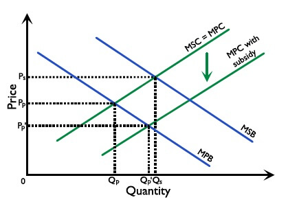
In Figure 2.8.19, when a subsidy is being imposed on consumption that creates positive externalities, the cost of production decreases and supply increases. This shifts the MPC to MPC + subsidy. The private market equilibrium is now at MPB = MPC + subsidy. The quantity of output consumed increases from \(Q_p\)to \(Q_p’\), which is closer to the social optimal level \(Q_s\).
The effectiveness of subsidies depends on the elasticity of demand and supply); if the demand is more inelastic than the supply, the government will need to spend a lot on subsidies to reduce underprovision/underconsumption. At times the MSB (or MSC) and its equivalent monetary value is hard to determine, for instance in the case of subsidies for the arts. In addition, the use of subsidies would place large informational demands on the government. The government needs to know the MPC and MSC (positive externality of production) or the MPB and MSB (positive externality of consumption) of the private market to set the correct level of subsidies, but it is often difficult and costly to obtain the information. Subsidies also add to the government budget burden.
Singapore’s universal healthcare system is a mixed financing system, combining a public statutory insurance system, MediShield Life, which covers large bills arising from hospital care, with patients paying premiums, deductibles, co-insurance, and any costs above the claim limit, plus government subsidies and a compulsory medical savings account.
Hospitalisation, outpatient care, and long-term care are heavily subsidised; for example, Singaporeans can get subsidies of up to 80% for their bills at public hospitals. Lower-income families also get additional help from the government; lower- to middle-income families get up to 50% subsidies on their MediShield Life premiums, for example. The amount of direct government subsidies for healthcare given to Singaporeans has doubled from around $2.6 billion to around $5.6 billion between 2010 and 2016.
Government provision
When goods and services have very large positive externalities, such that they would be heavily underprovided in private markets, governments may choose to directly provide the goods and services. e.g. government-run primary schools and health clinics. While direct provision by the government can ensure that the goods or services are provided at the socially optimal level, without an effective managing mechanism, government provisions may be more expensive than private provisions, and government spending may be displaced from other areas.
In Hong Kong, the Department of Health provides a free comprehensive childhood immunisation programme. This aims to ensure that infants and children are protected from serious infectious diseases, and that uptake of the vaccination programme is higher than it would be if the government were not providing it directly.
The table summarises the Department of Health schedule dated 9 October 2024. It illustrates government provision at that date; birth-cohort arrangements are explained below.
PCV15 is the 15-valent pneumococcal conjugate vaccine. MMRV combines measles, mumps, rubella and varicella protection. Department of Health schedule (9 October 2024)
| Age | Vaccination |
|---|---|
| Newborn | BCG (against tuberculosis)
Hepatitis B (first dose) |
| 1 month | Hepatitis B (second dose) |
| 2 months | DTaP-IPV (first dose); PCV15 (first dose) |
| 4 months | DTaP-IPV (second dose); PCV15 (second dose) |
| 6 months | Hepatitis B (third dose)
DTaP-IPV (third dose) |
| 12 months | MMR (first dose); varicella (first dose); PCV15 (booster) |
| 18 months | DTaP-IPV (booster); MMRV (second dose, for children born on or after 1 July 2018) |
| Primary 1 | DTaP-IPV (booster); MMRV for children born 1 January 2013–30 June 2018 |
| Primary 5 | 9-valent HPV (first dose, girls) |
| Primary 6 | Reduced-dose diphtheria and pertussis / tetanus / inactivated polio (booster); 9-valent HPV (second dose, girls) |
Summary of the advantages and disadvantages of regulatory policies and market based policies
| Advantages | Disadvantages | |
|---|---|---|
| Regulation |
|
|
| Taxes |
|
|
| Subsidies |
|
|
| Tradable permits |
|
|
| Education/awareness |
|
|
| Direct provision |
|
|
| International agreements |
|
|
| Collective self-governance |
|