2.6 Price elasticity of supply (PES)
Price elasticity of supply (PES)
The price elasticity of supply measures the responsiveness of quantity supplied to a change in price, along a given supply curve.
\( PES = \frac{\% \Delta Qs }{\% \Delta P} \)
According to the law of supply, when there is an increase in price, the quantity supplied will increase. Therefore, in the formula of PES, when the denominator is positive, the numerator will be positive, and the mathematical value of the PES is positive.
Implications of values of PES
The value of the PES tells us how responsive the quantity supplied is to a change in price. To interpret the implication of the PES value, let us consider the following example:
Given the supply schedule for good X as follows, what is the PES for good X and what does the PES value imply?
| Price | Quantity supplied | |
|---|---|---|
| Old | $5 | 10 |
| New | $7 | 15 |
\( \% \Delta Qs = \frac{15-10}{10} \times 100\% = \frac{5}{10} \times 100\% = +50\% \)
\( \% \Delta P = \frac{7-5}{5} \times 100\% = \frac{2}{5} \times 100\% = +40\% \)
\( PES = \frac{\% \Delta Qs}{\% \Delta P} = \frac{+50\%}{+40\%} = +1.25 \)
The PES sign shall be positive because of the positive relationship of price and quantity supplied.
The PES number 1.25 means the numerator is greater than the denominator. % change in Qs is greater than the % change in P. We say that Qs is responsive to a price change, or the supply is price elastic.
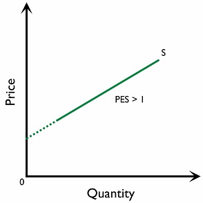
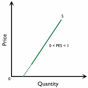
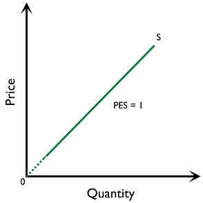
Hence the implications of the values of PES can be summarised in Table 1.2.3
Table 1.2.3 Implications of the values of PES
| Price Elasticity of supply | PES value | Meaning | Diagram |
|---|---|---|---|
| Elastic | PES > 1 | %Δ in Qs > %Δ in P | Figure 2.6.1 |
| Inelastic | 0 < PES < 1 | %Δ in Qs < %Δ in P | Figure 2.6.2 |
| Unit elastic | PES = 1 | %Δ in Qs = %Δ in P | Figure 2.6.3 |
| Perfectly inelastic | PES = 0 | %Δ in Qs = 0 | Figure 2.6.4 |
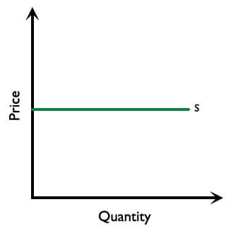
| Perfectly elastic | PES \( \rightarrow \infty \) | %Δ in Qs \( \rightarrow \infty \) | Figure 2.6.5 |
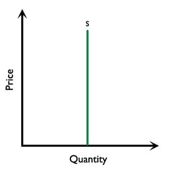
A perfectly inelastic supply curve (a vertical line) represents goods with fixed supply in the short run, such as agriculture products and seats in a stadium.
Determinants of PES
1) Time
Whether the suppliers have enough time to react to a price change is important for determining the elasticity of supply. In the short run, some factors are fixed; producers cannot increase or decrease their output level when there is an increase or decrease in demand, as not all adjustments are made possible. The supply is rather inelastic. In the long run, all factors are variable and all adjustments can be made; firms are able to adjust their output level according to the price change, thus the supply tends to be more elastic.
2) Rate at which costs increase
Supply is likely to be inelastic if total costs rise quickly when the producer tries to increase supply; in this case, the price of the good would have to rise significantly to make additional supply worthwhile. If total costs do not rise quickly, the producer can raise the quantity supplied more cheaply in response to an increase in price in order to make greater profits, and supply will be price elastic.
Factors which assist in preventing a significant rise in costs include:
- Mobility of factors of production
- Unused capacity
Producers are able to supply a variety of goods that require the same kinds of input. If the factors of production are mobile, firms can switch the resources to meet the increase in demand for certain products. The output level can be adjusted easily and the supply tends to be more elastic.
If the firm is operating far below the unused capacity, meaning it has a buffer of unused capacity, it is more possible for the firm to adjust their output level by working on its unused capacity when the price changes. The PES will be higher.
3) Ability to hold stock
If the firm has the ability to hold stock, the firm can raise their output level when there is an increase in the price level of the good. The PES will be higher. However, constrained by the nature of goods, it is hard to hold the stock for perishable products like flowers, hence their PES is lower.
PES for primary commodities and manufactured products
The PES for primary commodities such as coffee and wheat is relatively low, as its production is constrained by the long planting time lag and the low ability to hold stock. It is hard to adjust the output level within a short period of time.
Even for non-agricultural commodities such as oil, the PES is low as well. Though firms may have a higher ability to hold stock, the long extraction time and requirement of skilled workers in extraction also make it difficult for firms to adjust the output level in response to the demand change.
On the other hand, the PES for manufactured products, such as cars, is relatively high. The main factors of production are labour and capital, which can be increased in a short period of time. The competition among firms is keen, and market supply will respond quickly to the demand change.