2.5 Elasticities of demand
Elasticity is a measure of the responsiveness of something to a change in one of its determinants.
Price Elasticity of Demand (PED)
The Price Elasticity of Demand measures the responsiveness of quantity demanded to a change in price, along a given demand curve.
\( PED= \frac{ \% \Delta Qd }{\% \Delta P} \)
\( \% \Delta Qd= \frac{Qd(new)-Qd(old)}{Qd(old)} \times 100 \% \)
\( \% \Delta P=\frac{P(new)-P(old)}{P(old)} \times 100 \% \)
For a downward-sloping demand curve, price and quantity demanded move in opposite directions, so the signed value of PED is negative. When classifying demand as elastic, unit elastic or inelastic, we use the absolute value of PED: greater than 1, equal to 1 or less than 1 respectively.
The value of PED tells us how responsive quantity demanded is to a change in price. To interpret the implication of the PED value, let us consider the following example:
Given the demand schedule for good X, what is the PED value for good X and what does the PED value imply?
| Price | Quantity demanded | |
|---|---|---|
| Old | $5 | 10 |
| New | $6 | 5 |
\( \% \Delta Qd= \frac{Qd(new)-Qd(old)}{Qd(old)} \times 100 \% \)
\( = \frac{(5 - 10)}{10} \times 100\% = \frac{- 5}{10} \times 100\% = -50\% \)
\( \% \Delta P= \frac{P(new)-P(old)}{P(old)} \times 100 \% \)
\( = \frac{(6 - 5)}{5} \times 100\% = \frac{1}{5} \times 100\% = 20\% \)
\( PED = \frac{\% \Delta Qd }{\% \Delta P } = \frac{-50\%}{20\%} \) = -2.5
The PED sign shall be negative because of the inverse relationship of price and quantity demanded.
The PED number 2.5 means the numerator is greater than the denominator. The % change in Qd is greater than the % change in price. We say that the quantity demanded is responsive to a price change, or demand is price elastic.
A common error is to say the change in Qd is larger than the change in price when the demand is elastic. The correct way of saying it should be: the % change in Qd is larger than % change in price, or we can also say a small change in price leads to a proportionally greater change in Qd.
Hence the implications of the values of the PED can be summarised in Table 2.5.1.
Table 2.5.1: Implications of the values of PED
| Price Elasticity of demand | PED value | Meaning | Diagram |
|---|---|---|---|
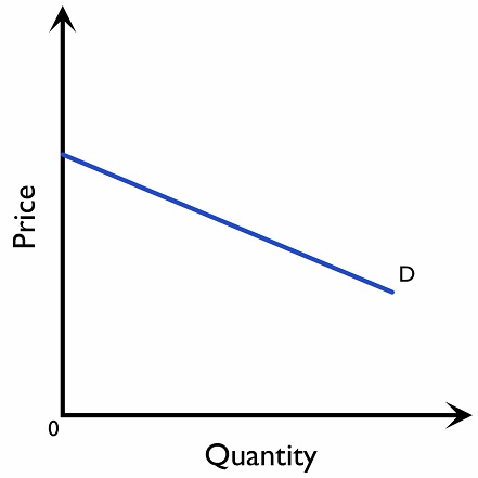
| Elastic | PED > 1 | %Δ in Qd > %Δ in P | Figure 2.5.1 |
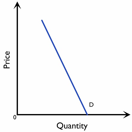
| Inelastic | 0 < PED < 1 | %Δ in Qd < %Δ in P | Figure 2.5.2 |
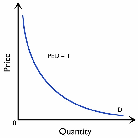
| Unit elastic | PED = 1 | %Δ in Qd = %Δ in P | Figure 2.5.3 |
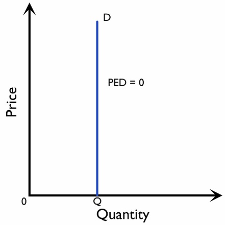
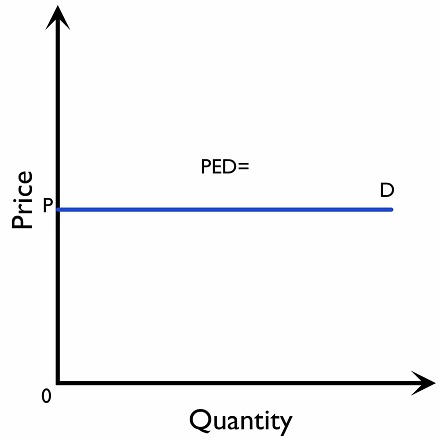
| Perfectly inelastic | PED = 0 | %Δ in Qd = 0 | Figure 2.5.4 |
| Perfectly elastic | PED \( \rightarrow \) \( \infty \) | %Δ in Qd \( \rightarrow \) \( \infty \) | Figure 2.5.5 |
Determinants of PED
1) Availability of substitutes
Goods with close substitutes tend to have a more elastic demand as consumers are able to find substitutes when there is a change in price. For example, if the price of one newspaper increases, the consumer can switch to another newspaper, therefore, the demand for independent newspapers is likely to be elastic. On the other hand, goods with few substitutes will have a more inelastic demand.
2) The proportion of income spent on a good
Goods that take up a small proportion of income will have an inelastic demand even when there is a high percentage change in price. For example, a 20% increase in the price of a dress from $100 to $120 takes up a relatively small proportion of income. On the other hand, if consumers spend a large proportion of income on a product, such as a dress that costs $2000, then a similar 20% increase in the price will mean that the dress now costs $2400. This takes up a relatively larger proportion of income, meaning that its demand will be more elastic as it will have a bigger impact on the amount of income spent.
3) Degree of necessity
Goods that are considered as a 'must have' item will have an inelastic demand, such as food, as the consumption can hardly be reduced even if the price rises. On the other hand, goods that are not essential (e.g. luxury products) will have a more elastic demand as consumers can respond to the higher price by making the purchase later. Nevertheless, some consumers consider luxurious products not essential but others may, and ultimately, the PED depends on the individual's preferences.
4) Time
Demand is usually inelastic in the short run as it takes time for people to find substitutes. In the long run, demand for goods tends to be more elastic.
Calculate the PED between two designated points
Consider the linear demand curve below (Figure 2.5.6):
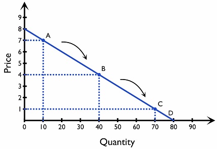
\[PED \; from \; A \; to \; B = \frac{\% \Delta Qd }{\% \Delta P} = \frac{ \frac{(40-10)}{10} \times 100\%}{ \frac{(4-7)}{7} \times 100\%} = \frac{300\%}{- 43\%} = -7 \]
\[ PED \; from \; B \; to \; C = \frac{\% \Delta Qd }{\% \Delta P} = \frac{ \frac{(70-40)}{40} \times 100\%}{ \frac{(1-4)}{4} \times 100\%} = \frac{75\%}{- 75\%} = -1 \]
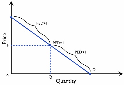
From the above example, we see that two different points on the same demand curve will have a different price elasticity of demand. In reality, the upper portion of the demand curve has a more elastic demand, while the lower portion of the demand curve has a more inelastic demand. Figure 2.5.7 shows different PED levels in various portions on a linear demand curve.
Calculation of PED is different from the calculation of a slope. The PED value varies along a linear demand curve. The slope from A to B is equal to the slope from B to C as they are all situated on the same straight line. However, PED from A to B is different from PED from B to C. Therefore, PED ≠ slope.
Relationship between PED and total revenue
Total revenue means the total money received by a firm from the sale of a particular quantity of output and is equal to price times quantity sold. According to the law of demand, when the price rises, the quantity demanded decreases. The change in total revenue depends on the price elasticity of demand (PED).
When demand is elastic, an increase in price from \(P_1\) to \(P_2\) will cause a higher percentage decrease in quantity demanded from \(Q_1\) to \(Q_2.\) The gain in total revenue from a price increase is lower than the loss in revenue from a quantity decrease. Total revenue therefore decreases. (Figure 2.5.8)
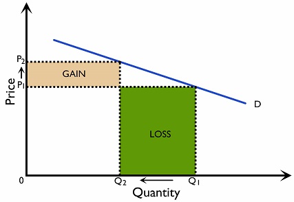
When demand is inelastic, an increase in price from \(P_1\) to \(P_2\) will cause a lower percentage decrease in quantity demanded from \(Q_1\) to \(Q_2\). The gain in total revenue from price increase is larger than the loss in revenue from quantity decrease. Total revenue therefore increases. (Figure 2.5.9)
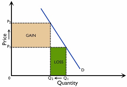
Table 2.5.2 Impacts of price change on total revenue under different PED values
| Δ in P | PED | Implications | Δ in TR |
|---|---|---|---|
| ↑ | Elastic PED > 1 | Loss from ↓Q > Gain from ↑P | ↓ |
| ↓ | Gain from ↑Q > Loss from ↓P | ↑ |
|
| ↑ | Inelastic PED < 1 | Loss from ↓Q < Gain from ↑P | ↑ |
| ↓ | Gain from ↑Q < Loss from ↓P | ↓ |
|
| ↑ | Unit elastic PED = 1 |
Loss from ↓Q = Gain from ↑P | - |
| ↓ | Gain from ↑Q = Loss from ↓P | - |
Importance of PED to firms
One of the firm’s objectives is to maximise revenue. A firm can maximise revenue by setting different price levels. Assume the demand for cigarettes is inelastic and there is an increase in price. The quantity demanded falls proportionally less than the increase in price. The gain from the increase in price is larger than the loss from the decrease in quantity demanded. The firm can increase the total revenue by raising the price of products with inelastic demand.
Importance of PED to the government
PED can help governments determine the size of indirect taxes being imposed. For instance, if the government wants to discourage smoking, and if the demand for cigarettes is inelastic, the size of indirect tax on cigarettes has to be big enough to achieve the results of reducing cigarette consumption.
Reasons why the PED for primary commodities is generally lower than the PED for manufactured products
Primary commodities are raw materials such as cotton or coffee; these are necessities to those who buy them, who tend to be manufacturing industries who need them as raw materials to produce processed products. They therefore have inelastic demand as there are few substitutes available for the manufacturing process.
However, demand for manufactured goods tends to be price elastic as there are more substitutes available to consumers.
Income elasticity of demand (YED)
Income elasticity of demand (YED) measures the responsiveness of quantity demanded to a change in income.
\( YED = \frac{\% \Delta Q_d \; A }{\% \Delta Income} \)
The sign (\( + \) or \( - \))
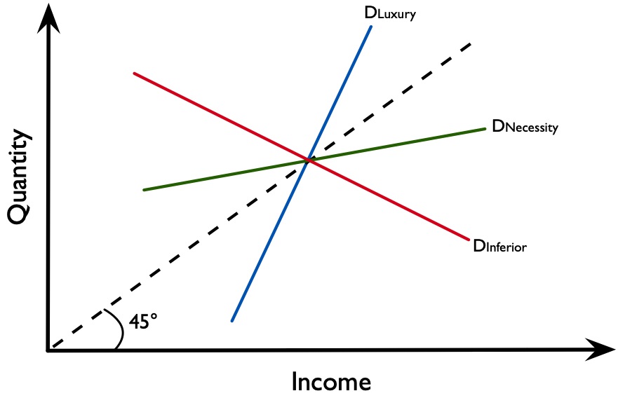
If the YED is positive, the good is a normal good. As income increases, quantity demanded increases and vice versa.
If the YED is negative, the good is an inferior good. As income increases, quantity demanded decreases and vice versa.
The absolute value of YED
Goods which have YED < 0 are called ‘inferior goods’; the demand for them decreases as income increases. These are goods which people start to switch their expenditure away from as their income increases, for example people may stop buying cheap clothes and switch to more expensive brands.
If 0 < YED < 1, an increase in income will lead to a proportionately smaller increase in demand, and the good is a ‘necessity’ good for which the demand changes little as income rises. An example is milk; even if income rises, people will not feel that they need to buy more milk.
If YED > 1, an increase in income will lead to a proportionately larger increase in demand, and the good is a ‘luxury’ good. When people have enough income to satisfy their basic needs, they start to purchase things that are ‘wants’ rather than essentials. An example would be foreign holidays.
The graph 2.5.10 below shows the Engel curves of different types of goods.
The average income in an area changes from £500 per week to £550 per week. Following the change, the local ice cream vendor sells 1,500 ice creams per week, up from 1,200 ice creams per week.
Calculate ice cream’s YED value:
\( YED = \dfrac{ \%\;change\;in\;Q}{\%\;change\;in\;Y}\)
Percentage change in quantity demanded:
\(\dfrac{1,500-1,200}{1,200}\times 100\%=25\%\)
Percentage change in income:
\(\dfrac{550-500}{500}\times 100\%=10\%\)
\(YED=\dfrac{\%\delta Q}{\%\Delta Y}=\dfrac{25}{10}=2.5\)
Given that the sign of the YED is positive, this means that ice cream is a normal good.
As YED value (2.5) is greater than 1, ice cream’s YED is elastic.
The importance of YED
YED is important for:
- Decision-making by firms: A knowledge of YED can help firms to plan which markets to enter and which products to sell. When the economy is expanding, the demand for goods with high YED increases, and the markets for those goods grow quickly. A firm will therefore try to be aware of the YED of their products and the incomes of their target consumers to make the most of opportunities. Producers may also manufacture different versions of their goods in order to appeal to customers of different incomes. If the economy goes into a recession, they will increase production of inferior goods, whose demand increases as income falls.
- For explaining sectoral changes in the structure of the economy: Production is split into three sectors: primary (agricultural), secondary (manufacturing), and tertiary (services). ‘Sectoral change’ is the shift in the relative share of national output and employment in each of these sectors over time. As countries grow over time, the proportion of the economy that is produced in the secondary and tertiary sectors relative to the primary sector is likely to grow. This can be explained using YED: as incomes increase, the demand for primary goods is likely to not increase much as they are income inelastic. This extra income is therefore spent on manufactured products which are income-elastic. As the country develops further, the same mechanism will lead to growth of the service sector. Tertiary goods, like services, tend to have a higher YED, so there will be faster growth in the tertiary sector when the economy grows. For example, consumers are unlikely to buy convenience services such as dog walking when their income is low and they are focussed mainly on buying necessities; however, when their income grows and they are able to satisfy their need for agricultural goods and manufactured goods, they will start to purchase tertiary goods.