2.3 Competitive market equilibrium
Demand and supply curves forming a market equilibrium
When we put demand and supply together, the market force automatically adjusts the price until the quantity demanded is equal to the quantity supplied. This is the equilibrium price, known as the market clearing price, where there is no tendency for the price to change and the quantity demanded \((Q_d)\) is equal to the quantity supplied \((Q_s)\).
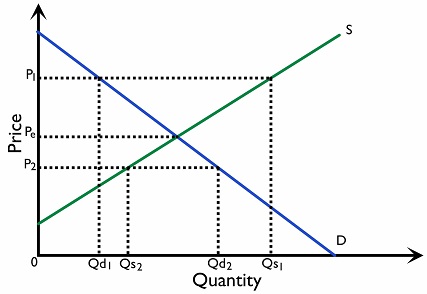
In Figure 2.3.1, when the price is at \(P_1\), the price is so high that many producers want to produce more but few consumers demand it. The quantity supplied \((Q_{s_1})\) is larger than the quantity demanded \((Q_{d_1})\), there is an excess supply/ surplus of \((Q_{s_1} - Q_{d_1})\) units. With the surplus, producers are willing to lower the price to get rid of the surplus, thus there is a tendency for the price to fall.
When the price is at \(P_2\), the price is so low that many consumers want to buy the good but few producers are willing to produce it. The quantity demanded \((Q_{d_2})\) is larger than the quantity supplied \((Q_{s_2})\), and there is an excess demand/shortage of \((Q_{d_2} - Q_{s_2})\) units. With the shortage, consumers are willing to pay a higher price, thus there is a tendency for the price to rise.
When the price is at \(P_e\), quantity demanded equals quantity supplied; there is neither excess demand nor excess supply and we say that the market is cleared. \(P_e\) is the equilibrium price.
Changes in Equilibrium
Shift of the demand curve
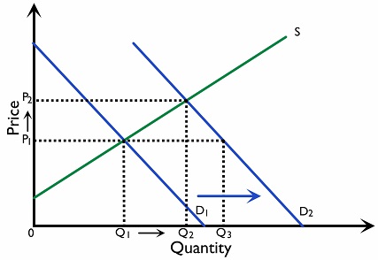
In Figure 2.3.2, when the demand increases and the demand curve shifts to the right from \(D_1\) to \(D_2\), there will be an excess demand of \((Q_3 - Q_1)\) units at the original price \(P_1\). The price will have a tendency to rise. The equilibrium price and quantity will be increased from \(P_1\) to \(P_2\) and \(Q_1\) to \(Q_2\) respectively.
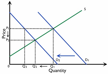
In Figure 2.3.3, when demand decreases and the demand curve shifts to the left from \(D_1\) to \(D_2\), there will be an excess supply of \((Q_1-Q_3)\) units at the original equilibrium price \(P_1\). The price will have a tendency to fall. The equilibrium price and quantity will decrease from \(P_1\) to \(P_2\) and \(Q_1\) to \(Q_2\) respectively.
A shift of the supply curve
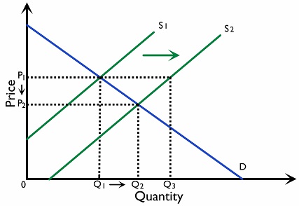
In Figure 2.3.4, when the supply increases and the supply curve shifts to the right from \(S_1\) to \(S_2\), there will be an excess supply of \((Q_3 - Q_1)\) units at the original price \(P_1\). The price will have a tendency to fall. The equilibrium price will fall from \(P_1\) to \(P_2\) and the quantity will rise from \(Q_1\) to \(Q_2\).
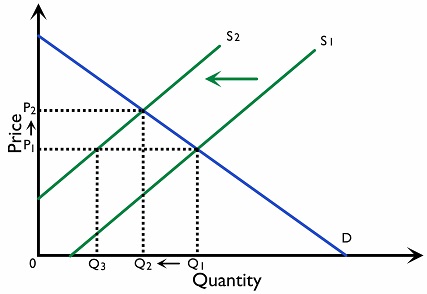
In Figure 2.3.5, when supply decreases and the supply curve shifts to the left from \(S_1\) to \(S_2\), there will be an excess demand of \((Q_1 - Q_3)\) units at the original equilibrium price \(P_1\). The price will have a tendency to rise. The equilibrium price will rise from \(P_1\) to \(P_2\) and the quantity drops from \(Q_1\) to \(Q_2\).
A shift of both demand and supply curves
When demand and supply shift simultaneously, one effect can be determined from the directions of the shifts, while the other depends on their relative sizes. If both increase, equilibrium quantity rises; if both decrease, quantity falls. In each case, the price change is uncertain. If demand increases while supply decreases, price rises; if demand decreases while supply increases, price falls. In these cases, the quantity change is uncertain. The table below summarises these effects.
| Change in demand (D) and supply (S) | Effects on price (P) and quantity (Q) |
|---|---|
| D ↑ and S ↑ | P uncertain and Q ↑ |
| D ↑ and S ↓ | P ↑ and Q uncertain |
| D ↓ and S ↑ | P ↓ and Q uncertain |
| D ↓ and S ↓ | P uncertain and Q ↓ |
Functions of the price mechanism
Scarcity refers to the case when limited resources are not enough to satisfy unlimited human wants. It is the fundamental economic problem that all societies face. As a result, choices have to be made on how we allocate resources to fulfil human wants.
Opportunity cost refers to the next best alternative foregone. It arises whenever people make choices. Resources have alternative use: when we allocate a resource to one use, we have to sacrifice the alternative uses of the resource.
Signalling and incentive functions
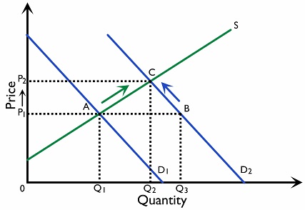
We can illustrate the signalling and incentive function of price using a demand-supply diagram. In Figure 2.3.6, the market equilibrium price and quantity for good X is at \(P_1\) and \(Q_1\), meaning scarce resources have been allocated to produce \(Q_1\) units of good X.
Suppose the demand for good X increases, then there will be an excess demand of (AB) units at \(P_1\), which would drive up the price to \(P_2\). This rise in price acts as a signal to producers of the market situation and provides an incentive for them to supply more. Therefore, the quantity supplied increases from \(Q_1\) to \(Q_2\). At the same time, a rise in price also signals consumers to cut back their consumption and lower their quantity demanded.
As more quantity is produced, more resources have to be allocated for the increase in production. This process involves a reallocation of resources and is determined by the invisible hand in the market without government intervention.
Rationing function
The price mechanism allocates scarce resources. In a market economy, those who are willing and able to pay would receive the resources. If the quantity demanded for a good is greater than the quantity supplied at a given price, prices will be higher and the goods will be bought by consumers who are willing and able to pay the higher price.
Consumer and producer surplus
Consumer Surplus
Consumers demand for a good when the benefit (or value) derived from consumption is greater than or equal to the price paid for the good.
There are two ways to look at the demand curve:
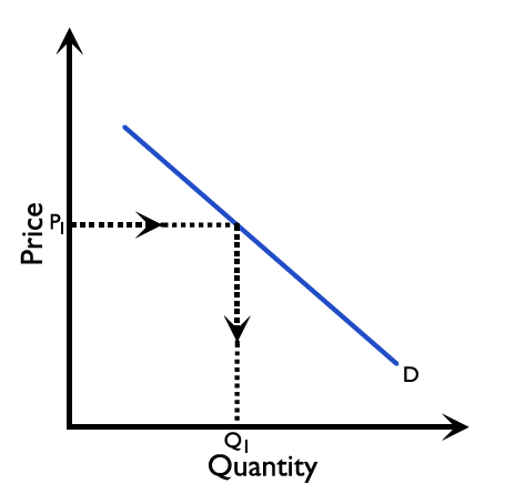
1) The demand curve shows the quantity consumers want to consume at different prices. For example, when the price is at \(P_1\), consumers want to buy at \(Q_1\). (Figure 2.3.7)
2) The demand curve also shows the maximum price consumers are willing and able to pay at different units. For example, the maximum amount the consumer is willing and able to pay for the \(Q_1\) unit is at \(P_1\) (Figure 2.3.8)
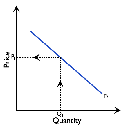
The vertical distance to a demand curve measures the marginal benefit (MB) enjoyed by the consumers for that unit, so the demand curve is also the marginal benefit (MB) curve.
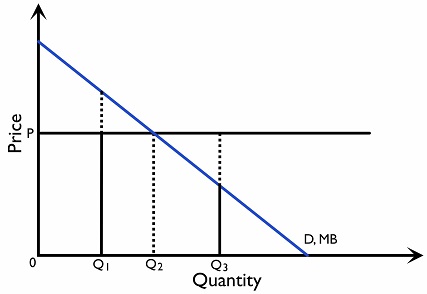
Each consumer is subjected to maximise gain. Gain is maximised if the value of an additional unit consumed is greater than the actual price paid to obtain the unit. Figure 2.3.9 assumes the price is at \(P\), and the consumer is consuming at \(Q_1\). The consumer will continue to consume more as the marginal benefit is still larger than the price, and potential gain can be captured by consuming more. However, the consumer shall not consume more than \(Q_2\) units. It is because, at units beyond \(Q_2\), e.g. at \(Q_3\), the marginal benefit of this unit is less than the actual price paid in obtaining it. Consuming this unit reduces the consumer’s gain. Therefore, the consumer maximizes the gain when consuming up to the unit where the marginal benefit equals the actual price, which is at \(Q_2\).
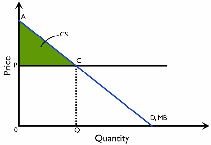
Consumer surplus is the amount an individual is willing and able to pay minus the actual amount he has to pay for a given quantity of the good.
Suppose that you are willing to pay $35 for a cup of coffee and you only pay $30; the consumer surplus is ($35 – $30 = $5).
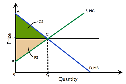
In Figure 2.3.10, for the amount Q, the consumer is actually willing and able to pay for the area \((0ACQ)\), yet he only needs to pay for the area \((0PCQ)\). Therefore, the consumer surplus is the area (APC), which is the difference between area \((0ACQ)\) and area \((0PCQ)\).
Producer Surplus
Producers who sell a good must receive a value that is greater than or equal to the production cost. The supply curve shows the quantity suppliers are willing and able to supply at different prices. In other words, we can define the price as the minimum amount a supplier is willing and able to sell for a particular unit. This minimum amount is the cost of producing that extra unit, the marginal cost. Therefore, the supply curve is actually the marginal cost (MC) curve.
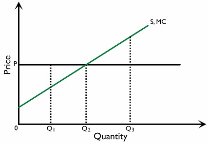
Each supplier is subjected to maximise gain. Gain is maximised if the price of an additional unit is greater than the marginal cost in producing the unit. Figure 2.3.11 assumes that the price is at \(P\), and the \(Q_s\) is at \(Q_1\). Suppliers will continue to supply more as the price is still larger than the marginal cost, and the potential gain can be captured by producing more. However, the producer shall not supply more than \(Q_2\) units. It is because, at units beyond \(Q_2\), the marginal cost is higher than the actual price in the market. Producing this unit reduces the producer’s gain. Therefore, the producer maximizes the gain when supplying up to the unit where the marginal cost equals the price.
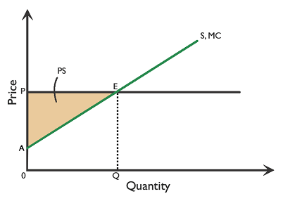
Producer surplus is the actual amount that a producer receives for selling their good minus the lowest amount for the producer to offer a given quantity of a good.
In Figure 2.3.12, for the amount Q, the minimum amount the producer needs to receive is the area \((0AEQ)\), but the producer actually receives the area \((0PEQ)\). Therefore, the producer surplus is the difference between the area \((0AEQ)\) and the area \((0PEQ)\), which is the area \((APE)\).
Allocative efficiency
Total Social Surplus is defined as the sum of the consumer surplus and the producer surplus.
Figure 2.3.13 shows the market price P, consumer surplus is the area (APC) and the producer surplus is the area (BPC). Therefore, the total social surplus is equal to the area (ABC).
Allocative efficiency is achieved when it is impossible to reallocate resources where at least one person gains without making anyone worse off.
In Figure 2.3.14, the optimal quantity is at \(Q_2\) units. We shall see why \(Q_1\) and \(Q_3\) are not the optimal production levels.
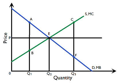
When the production level is at \(Q_1\), the marginal benefit (A) is higher than the marginal cost (B), which means the marginal cost of producing that unit is lower than what the consumers are willing and able to pay for that unit. Extra surplus area (ABE) can be captured by producing more. Therefore \(Q_1\) is not the optimal quantity.
When the production level is at \(Q_3\), the marginal cost (C) is higher than the marginal benefit (F), which means the marginal cost of producing that unit is higher than what the consumers are willing and able to pay for that unit. Society will suffer a loss of surplus equals to the area \((CEF)\) by producing at \(Q_3\). Therefore \(Q_3\) is not the optimal quantity.
Ultimately, at the optimal level \(Q_2\), the marginal benefit and marginal cost are equal, so that the total social surplus is maximised.