4.2 Types of trade protection
Tariff
A tariff is a tax imposed on imports. It can be on a specific or ad valorem basis. Both a specific and ad valorem tariff will shift the world supply curve upward. Figure 4.2.1 shows the effect of a tariff.
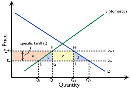
The demand (D) and supply (S) shown in the figure is the domestic demand and domestic supply for good A in country X. Assume country X is a small country and a price taker. The world price is at \(P_w\). Facing competition from imports, the domestic price of good A is at \(P_w\). At \(P_w\), the domestic producers are willing and able to supply at \(Q_1\), and consumers are willing and able to buy at \(Q_2\). The excess demand \((Q_2-Q_1)\) generated in the economy is filled up by imports. The world supply \((S_w)\) is a horizontal line at \(P_w\), indicating country X can consume up to any quantity at \(P_w\) and will not bring any change to the world price.
Suppose now a specific tariff of ($t) is imposed. The domestic price will rise from \(P_w\) to \((P_w + t)\). At \((P_w + t)\), the domestic production rises from \(Q_1\) to \(Q_3\), while the quantity demanded decreases from \(Q_2\) to \(Q_4\). The excess demand \((Q_4 - Q_3)\) is filled up by imports. There is a reduction in imports from \((Q_2 - Q_1)\) to \((Q_4 - Q_3)\). The effects of the tariff on different stakeholders are summarised in Table 4.2.2.
Table 4.2.2 The effects of a tariff to different stakeholders
| Stakeholders | Gain/Loss | Explanation |
|---|---|---|
| Domestic producers | Gain |
Revenue of domestic producer increases from \((P_w \times Q_1)\) to \((P_w+t) \times Q_3\)
Increase in producer surplus by area a |
| Foreign producers | Loss | The import revenue decreases from \((Q_2 - Q_1) \times P_w\) to \((Q_4 - Q_3) \times P_w\) |
| Consumers | Loss |
Face higher price level at \(P_w + t\)
Decrease in consumer surplus by area (a + b + c + d) |
| Government | Gain | Increase in tariff revenue by area c |
| Society | Loss | A net welfare loss of (b + d) |
The area b can be seen as production inefficiency. It is because the economy shifts purchases from efficient overseas firms to inefficient domestic firms for the quantity of \((Q_3 - Q_1)\). The production cost to produce \((Q_3 - Q_1)\) units by domestic firms is equal to the area \((Q_1EFQ_3)\), which can be originally produced by more efficient overseas firms at \((Q_1EGQ_3)\). The extra cost paid is the area b.
The area d can be seen as consumption inefficiency. The unit \((Q_2 - Q_4)\) is now not consumed because of the imposition of the tariff. However, we can see that \((Q_2 - Q_4)\) unit is worth \((HJQ_2Q_4)\) to consumers and they can be originally purchased at \((Q_2Q_4IJ)\). The consumer surplus equivalent to area d has now dissipated.
Calculations on the effects of imposing a tariff
Assume that the world supply is plotted as a horizontal line \(S_w\). The world price is at \(P_w = $2\). A specific tariff of $1 is imposed, the world supply curve shifts from \(S_w\) to \(S_w + tariff\) and the domestic price will rise from $2 to $3. (Figure 4.2.3)
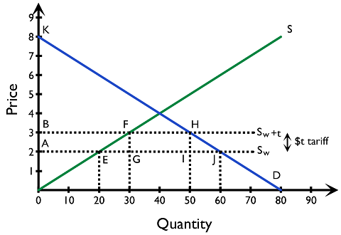
Students are required to know how to calculate the effects on different stakeholders of tariffs. The effects of the tariff are summarised in Table 4.2.4.
| Table 4.2.4 The effects of tariff | ||
|---|---|---|
| P (before tariff) | $2 | |
| P (after tariff) | $3 | |
| Domestic production (before tariff) | 20 | |
| Domestic production (after tariff) | 30 | |
| Consumption level (before tariff) | 60 | |
| Imports (before tariff) | EJ | 60 – 20 = 40 |
| Imports (after tariff) | FH | 50 – 30 = 20 |
| Consumption level (after tariff) | 50 | |
| Initial consumer surplus | Area AKJ | \( \frac{($8 - $2) \times 60 }{2} = $180 \) |
| New consumer surplus | Area BKH | \( \frac{($8 - $3) \times 50 }{2} = $125 \) |
| Loss in consumer surplus | Area ABHJ | $180 - $125 = $55 |
| Initial domestic producer surplus | Area 0AE | \( \frac{($2 - 0) \times 20 }{2} = $20 \) |
| New domestic producer surplus | Area 0BF | \( \frac{($3 - 0) \times 30 }{2} = $45 \) |
| Increase in domestic producer surplus | Area ABFE | $45 - $20 = $25 |
| Government’s tax revenue | Area FGHI | (50 − 30) units × $1 per unit = $20 |
| Welfare loss | Area EFG +Area HIJ | $55 – $25 - $20 = $10 |
Quota
A Quota is a limit on the quantity of imports placed by the government. Figure 4.2.5 shows the effects of a quota.
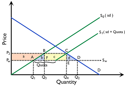
The demand (D) and supply (S) shown in the figure is the domestic demand and domestic supply for good A in country X. Assume the world price is at \(P_w\). Facing competition from imports, the domestic price of good A is at \(P_w\). At \(P_w\), the domestic producers are willing and able to supply at \(Q_1\), and consumers are willing and able to buy at \(Q_2\). The excess demand \((Q_2 - Q_1)\) generated in the economy is filled up by imports.
Suppose a quota of BC is imposed by the government so that no more than BC units of imports can be traded in the country. Now, the effective supply within the country becomes \(S_1\). The available quantity in the country is the domestic supply plus no more than BC units of imports. The price in domestic market rises from \(P_w\) to \(P_2\), domestic production increases from \(Q_1\) to \(Q_3\), imports reduced from \((Q_2 - Q_1)\) to \((Q_4 - Q_3)\) units.
Quota rent is the extra return from selling the permitted imports at the higher domestic price. It is represented by area c. Who receives it depends on the allocation of import licences: it may go to domestic importers, foreign exporters, or the government if licences are auctioned. This distinction matters when measuring domestic welfare.
Students are required to know how to calculate the effects on different stakeholders of quota. The effects of quota on different stakeholders are summarised in Table 4.2.6.
Table 4.2.6: The effects of quota
| Stakeholders | Gain/Loss | Explanation |
|---|---|---|
| Domestic producers | Gain |
Revenue of domestic producer increases from \((P_w \times Q_1)\) to \((P_2 \times Q_3)\)
Increase in producer surplus by area a |
| Foreign producers | Gain/Loss |
The import revenue changes from \((Q_2 - Q_1) \times P_w\) to \((Q_4 - Q_3) \times P_2\)
*Assume that the quota rent goes to foreign producers |
| Consumers | Loss | Decrease in consumer surplus by area (a + b + c + d) |
| Government | Gain/Loss | Depends on how the quota is allocated |
| Society | Loss | Domestic welfare falls by (b + c + d) under the stated assumption that foreign producers receive the quota rent. If the rent remains in the domestic economy, domestic welfare falls by (b + d). In this small-country model, the global efficiency loss is (b + d); area c is a transfer abroad rather than a global loss. |
Calculations on the effects of imposing a quota
The world supply is plotted as a horizontal line \(S_w\). The world price is at \(P_w = $2\). Suppose a quota of 20 units is imposed, the supply curve shifts from \(S_0\) to \(S_1\) at price level above \(P_w\). The domestic price will rise from $2 to $3. (Refer to Figure 4.2.7) The effects of quota are summarised in Table 4.2.8.
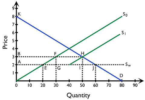
Although the supply curve shifts to the right, the domestic supply has not increased. It is because the domestic producers’ willingness and ability to sell has not been changed.
Who receives the quota rent? Consumers lose $55 and domestic producers gain $25. If foreign exporters receive the $20 rent, domestic welfare falls by $55 − $25 = $30. If the rent stays with domestic importers or the government, domestic welfare falls by $55 − $25 − $20 = $10. The two deadweight-loss triangles total $10 in either case; the remaining $20 is a transfer between countries.
| Table 4.2.8. The effects of quota |
|
|
|---|---|---|
| P (before quota) | $2 | |
| P (after quota) | $3 | |
| Domestic production (before quota) | 20 | |
| Domestic production (after quota) | 30 | |
| Imports (before quota) | EJ | 60 – 20 = 40 |
| Imports (after quota) | FH | 50 – 30 = 20 |
| Consumption level (before quota) | 60 | |
| Consumption level (after quota) | 50 | |
| Initial consumer surplus | Area AKJ | \( \frac{($8 - $2) \times 60 }{2} = $180 \) |
| New consumer surplus | Area BKH | \(\frac{(\$8-\$3)\times50}{2}=\$125\) |
| Loss in consumer surplus | Area ABHJ | $180 - $125 = $55 |
| Initial producer surplus | Area 0AE | \(\frac{(\$2-\$0)\times20}{2}=\$20\) |
| New producer surplus | Area 0BF | \(\frac{(\$3-\$0)\times30}{2}=\$45\) |
| Increase in producer surplus | Area ABFE | $45 - $20 = $25 |
| Quota rent | Area FGHI | (50 − 30) units × $1 per unit = $20 |
| Global deadweight loss (also domestic loss if quota rent stays domestically) | Area EFG + Area HIJ | $55 – $25 - $20 = $10 |
Subsidies
A subsidy is a grant provided by the government to firms aiming at lowering production costs and increasing output. Figure 4.2.9 shows the effects of the grants of a subsidy.
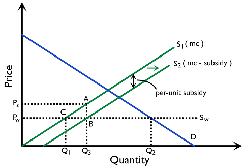
The demand (D) and supply (S) shown in the figure is the domestic demand and domestic supply for good A in country X. Assume the world price is at \(P_w\). Facing competition from imports, the domestic price of good A is at \(P_w\). At \(P_w\), the domestic producers are willing and able to supply at \(Q_1\), and consumers are willing and able to buy at \(Q_2\). The excess demand \((Q_2 - Q_1)\) generated in the economy is filled up by imports.
Suppose now a per-unit subsidy is granted by the government so that the production cost is lowered and the domestic supply curve shifts to the right from \(S_1\) to \(S_2\). Now, domestic production increases from \(Q_1\) to \(Q_3\) at \(P_w\), and imports are reduced from \((Q_2 - Q_1)\) to \((Q_2 - Q_3)\) units. The total quantity consumed by consumers is still the same at \(Q_2\), and there is an increase in the proportion of goods produced by domestic producers.
The grant of subsidy does not affect the world price and consumption quantity. The amount of subsidy grant is larger than the gain in producer surplus. In addition, governments also need to finance the grant through taxation. Ultimately, taxpayers pay the burden. There is a resource misallocation.
Students are required to know how to calculate the effects on different stakeholders of subsidies. The effects of subsidy on different stakeholders are summarised in Table 4.2.10
Table 4.2.10 The effects of subsidy
| Stakeholders | Gain/Loss | Explanation |
|---|---|---|
| Domestic producers | Gain | Increase in revenue from \((P_w \times Q_1)\) to \((P_s \times Q_3)\)
Increase in producer surplus of \(P_sP_wAC\) |
| Foreign producers | Loss | The import revenue decreases from \((Q_2 - Q_1) \times P_w\) to \((Q_2 - Q_3) \times P_w\) |
| Consumers | Unchanged | No change in consumption price and quantity |
| Government | Loss | The total subsidy expense equals \(P_sABP_w\) |
| Society | Loss | A net welfare loss of ABC |
Calculations on the effects of imposing a subsidy
The world supply is plotted as a horizontal line \(S_w\). The world price is at \(P_w = $2\). Suppose now a $2 per unit subsidy is granted. The domestic supply increases from S1 to S2. (Figure 4.2.11)
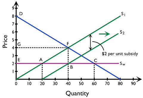
The effects of subsidy on different stakeholders are summarised in Table 4.2.12.
| Table 4.2.12 The effects of subsidy | ||
|---|---|---|
| P (before and after subsidy) | $2 | |
| Domestic production (before subsidy) | 20 | |
| Domestic production (after subsidy) | 40 | |
| Imports (before subsidy) | AC | 60 – 20 = 40
|
| Imports (after subsidy) | BC | 60 – 40 = 20
|
| Consumption level (before and after subsidy) | 60
|
|
| Consumer surplus (before and after subsidy) | Area CDE | \( \frac{($8 - $2) \times 60 }{2} = $180 \)
|
| Initial producer surplus | Area 0AE | \( \frac{($2 - 0) \times 20 }{2} = $20 \)
|
| New producer surplus | Area 0FG | \( \frac{($4 - 0) \times 40 }{2} = $80 \)
|
| Increase in producer surplus | Area AFGE | 80 - 20 = $60 |
| Government expense on subsidy | Area BFGE | 40 x $2 = $80 |
| Welfare loss | Area ABF | $80 - $60 = $20 |
Export subsidies
An export subsidy is a payment by the government to domestic producers for goods sold abroad. A per-unit export subsidy gives the producer a fixed payment for each unit exported.
Assume that the country is a small exporter and cannot influence the world price. There are no externalities. The subsidy is paid only on exports. Imports do not undercut the domestic price, and goods cannot be exported and re-imported simply to claim the subsidy.
The effect of an export subsidy
In Figure 4.2A, D and S represent domestic demand and supply. Before the subsidy, producers can sell their goods at the world price Pw. Domestic consumers buy Qd1 units and domestic producers supply Qs1 units. The difference, Qs1 − Qd1, is exported.
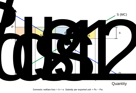
Suppose the government introduces an export subsidy of s per unit. A producer now receives Pw from the foreign buyer and s from the government for each unit exported. The total receipt is Pw + s. Producers will not sell the same good domestically for less than this amount when they can export it instead. The domestic price therefore rises to Ps = Pw + s.
At the higher domestic price, consumption falls to Qd2 and production rises to Qs2. Exports increase to Qs2 − Qd2. The increase in exports comes from both additional production and a reduction in the quantity available for domestic consumption.
The effects on different stakeholders
1) Domestic producers
Producers receive a higher price and sell a larger quantity. Producer surplus increases. They receive Ps on domestic sales and an equivalent amount, including the subsidy, on exports.
2) Domestic consumers
Consumers pay a higher price and buy fewer units. Consumer surplus falls. Some consumers who were willing to pay the world price are no longer willing or able to buy the good at Ps.
3) Government
The government pays the subsidy on the quantity exported after the policy. Its expenditure is s × (Qs2 − Qd2). The payment is not made on all domestic production. Financing this expenditure has an opportunity cost because the funds could be used for other purposes.
4) Society
The gain in producer surplus is smaller than the combined loss of consumer surplus and government expenditure. There are two sources of welfare loss.
For the extra units produced between Qs1 and Qs2, domestic marginal cost exceeds the world price received from foreign buyers. These units cost more resources to produce than the export revenue they earn. This is the production loss shown on the right of Figure 4.2A.
Consumption also falls between Qd2 and Qd1. For these units, domestic consumers' marginal benefit exceeds the world price. Exporting them instead of supplying domestic consumers sacrifices benefits greater than the receipts from abroad. This is the consumption loss shown on the left.
Areas in the export subsidy diagram
The band between Pw and Ps is divided into areas a to f in Figure 4.2A. These areas show changes in surplus and government expenditure. They do not represent the total consumer or producer surplus.
| Stakeholder | Change shown in Figure 4.2A | Explanation |
|---|---|---|
| Domestic consumers | Loss of a + c | Area a is the extra payment on the units still consumed. Area c is the loss of consumer surplus on the units no longer consumed. |
| Domestic producers | Gain of a + b + c + d + f | Areas a + b + c + d are the higher receipts on the original output. Area f is the extra surplus on the increase in production, after deducting its additional production cost. |
| Government | Expenditure of b + c + d + e + f | The subsidy is paid on exports after the policy. The rectangle has height Ps − Pw and width Qs2 − Qd2. |
| Domestic society | Net welfare loss of b + e | Area b is the consumption loss. Area e is the production loss. Both are losses of economic welfare, rather than transfers between domestic stakeholders. |
To find the net welfare effect, add the change in consumer surplus and producer surplus, then subtract government expenditure:
= −(a + c) + (a + b + c + d + f) − (b + c + d + e + f)
= −(b + e)
Some areas appear in more than one stakeholder's calculation because the same payment is a receipt for one party and an expense for another. These transfers cancel when the effects are added. The two welfare-loss triangles remain.
Calculations on the effects of an export subsidy
| Measure | Before the subsidy | After the subsidy |
|---|---|---|
| Domestic price | Pw | Ps = Pw + s |
| Domestic consumption | Qd1 | Qd2 |
| Domestic production | Qs1 | Qs2 |
| Exports | Qs1 − Qd1 | Qs2 − Qd2 |
| Revenue from foreign buyers | Pw(Qs1 − Qd1) | Pw(Qs2 − Qd2) |
| Total producer receipts, including subsidy | PwQs1 | PsQs2 |
| Government expenditure | 0 | s(Qs2 − Qd2) |
With straight-line demand and supply curves, the welfare loss is the sum of the two shaded triangles:
The fall in consumer surplus is ½s(Qd1 + Qd2). The increase in producer surplus is ½s(Qs1 + Qs2). Subtracting government expenditure from the net change in these surpluses gives the same welfare loss.
Calculations from an export subsidy diagram
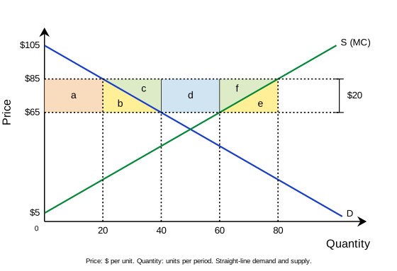
Figure 4.2B shows a small exporting country. Price is measured in dollars per unit, and quantity in units per period. Demand and supply are straight lines. The world price is $65 and the government pays a subsidy of $20 for each unit exported. The assumptions of Figure 4.2A still apply.
1) Read the prices and quantities
Before the subsidy, the domestic price is $65. Domestic consumption is 40 units and domestic production is 60 units. Exports are therefore 60 − 40 = 20 units.
After the subsidy, the domestic price rises to $85. Consumption falls to 20 units and production rises to 80 units. Exports increase to 80 − 20 = 60 units. The subsidy per unit can also be read as the vertical difference between the two price lines: $85 − $65 = $20.
2) Calculate the labelled areas
Areas a and d are rectangles. Areas b, c, e and f are triangles. Each has a height of $20; the relevant horizontal intervals are also 20 units.
| Area | Calculation | Value |
|---|---|---|
| a | ($85 − $65) × 20 | $400 |
| b | ½ × ($85 − $65) × (40 − 20) | $200 |
| c | ½ × ($85 − $65) × (40 − 20) | $200 |
| d | ($85 − $65) × (60 − 40) | $400 |
| e | ½ × ($85 − $65) × (80 − 60) | $200 |
| f | ½ × ($85 − $65) × (80 − 60) | $200 |
3) Calculate consumer surplus
The demand curve meets the price axis at $105. Consumer surplus is the triangle below demand and above the price paid, up to the quantity consumed.
After: ½ × ($105 − $85) × 20 = $200
Loss of consumer surplus = $800 − $200 = $600 = a + c
4) Calculate producer surplus
The supply curve meets the price axis at $5. Producer surplus is the area above supply and below the effective price received, up to domestic output. Producers receive $85 on domestic sales and $65 + $20 on exports.
After: ½ × ($85 − $5) × 80 = $3,200
Gain in producer surplus = $3,200 − $1,800 = $1,400
= a + b + c + d + f
5) Calculate government expenditure
The government pays the subsidy on 60 exported units. The 20 units sold to domestic consumers do not receive a subsidy.
= b + c + d + e + f
6) Calculate the welfare loss
= $600 + $1,200 − $1,400 = $400
Alternatively, welfare loss = b + e = $200 + $200 = $400
Before the subsidy, domestic welfare is $800 + $1,800 = $2,600. After the subsidy, it is $200 + $3,200 − $1,200 = $2,200. The reduction is again $400.
7) Distinguish revenue from surplus
| Measure | Before | After |
|---|---|---|
| Domestic consumer expenditure | $65 × 40 = $2,600 | $85 × 20 = $1,700 |
| Export receipts from foreign buyers | $65 × 20 = $1,300 | $65 × 60 = $3,900 |
| Total producer receipts, including subsidy | $65 × 60 = $3,900 | $85 × 80 = $6,800 |
Export receipts use the world price of $65 because this is the amount paid by foreign buyers. The government's subsidy is a separate payment. Producer receipts are not producer surplus: the cost represented by the area below the supply curve must also be considered.
In the import-competing production-subsidy model, consumers continue to buy at the world price and the subsidy is paid on domestic output. In this export-subsidy model, the domestic price rises and the subsidy is paid only on exports. The distinction changes both government expenditure and welfare.
Administrative barriers
Administrative barriers include forcing the importers to satisfy the product standards, health standards, pollution standards etc, set by the government. This may raise the cost for foreign producers and lower imports.