2.11 Market failure - market power
Market structure describes how the market is organised, in terms of the number of sellers and buyers, the entry and exit barriers, the level of market information available, the degree of price-setting power by firms, and the level of product differentiation. In the following sections - the costs, revenue and profit theories, as well as different market structures are analysed and explained.
Costs
Fixed cost and variable cost
Fixed costs are costs that remain constant as output increases. For instance, if a hawker has one food cart, and the cost of food carts does not change in relation to the quantity of food he sells.
Variable costs are costs that increase as output increases. For example, food is a variable cost in production. If the hawker sells more, more food is needed and hence the cost of food increases.
Note that a factor can be fixed or variable in various circumstances. The key is whether the factor varies with the output level.
Short run versus long run
Short run refers to production where there are both variable and fixed factors of production.
Long run refers to production where all factors of production are variable and no fixed factors are involved.
Long-run and short-run have nothing to do with time.
Explicit and implicit costs
The use of input involves costs, and each unit of output entails a cost. There are two kinds of costs: explicit costs and implicit costs.
Explicit cost is the type of cost one would find if looking through a firm’s accounting reports, for instance, rent paid for office premises or wages paid to employees.
Implicit cost is the value of the opportunity cost, or the next-best alternative forgone. For example, the firm could have let the office to some other firm, and receive rent. By using the office premises, it is giving up the rental income from the office space.
Short run production and cost curves
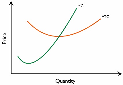
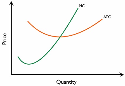
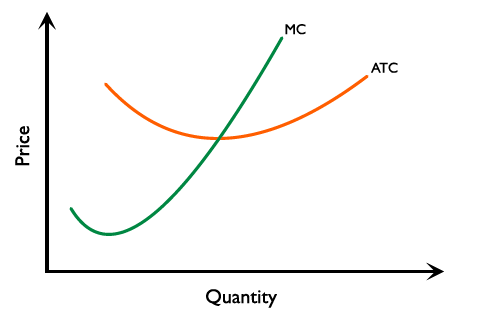
The short run cost structure of firms is guided by the law of diminishing marginal returns. According to the law of diminishing marginal returns, the marginal cost first decreases and then increases as output increases. It is therefore drawn in the shape of a “Nike swoosh”.
Average total cost (ATC) is drawn as a u-shape, and its shape can also be accounted to the presence of diminishing marginal returns. MC cuts the minimum point of the ATC. (Refer to Figure 2.11.0.1)
Long-run production and cost curve
The concept of long-run average cost (LRAC) is closely related to the concept of the short-run average cost (SRAC). Recall that in long-run production, all costs are variable, and any combination of factors can be used. Since one particular short-run average cost curve represents one particular combination of fixed factors/costs, any of these combinations can be chosen in the long-run. To get the LRAC curve, consider all possible short run cost curves. At any given quantity, the lowest short run average cost is marked as a point for the LRAC. Joining all the points of lowest short-run average cost over all quantities gives the LRAC.
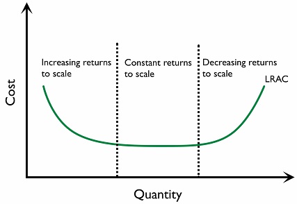
Economies of scale means the long run average cost decreases as a higher quantity of output is produced. This is illustrated in Figure 2.11.0.2. Firms can achieve these cost advantages due to:
(1) Purchasing economies
When producing large quantities, firms can buy in bulk or sign long-term agreements and obtain discounts, reducing the average cost of production.
(2) Financial economies
When firms are larger, banks may offer loans at lower interest rates owing to more collateral availability. Large firms can also have access to more financing instruments, such as issuing their own corporate bonds.
(3) Marketing economies
There are minimum charges for producing and broadcasting advertisements on TV or other media. When the quantity output is higher, marketing costs are spread over more output, resulting in a lower marketing cost per unit of output.
(4) Technological economies
Producing higher quantities of output enables the use of more powerful and efficient machinery, thus reducing average cost of production, which is only feasible at a certain minimum scale of output level.
Beyond a certain scale, LRAC might begin to increase with scale. In such a case there are diseconomies of scale, meaning an increase in output leads to an increase in the long run average cost, which can be caused by the following factors:
(A) Organisational complexity and communication breakdown
As firms become larger, they become increasingly difficult to manage. Communication between and within a large number of teams is more difficult than within a small number of teams. Manpower and effort is required to manage complex organisations with large numbers of workers, and this poses extra costs for the firm.
(B) Bureaucracy
As organisations grow, more rules might be introduced for guided decision-making, and is often a response to increasingly complex operations. However, rules also reduce flexibility, increasing average cost in communication. Bureaucracy in large organisations is also a source of diseconomies of scale.
Revenues
Total revenue, average revenue and marginal revenue
Total revenue (TR) is the total income that a firm receives by selling its products.
Total revenue (TR) = Price x Quantity
Since average revenue (AR) is TR divided by quantity. It follows that AR is equal to price.
Average revenue (AR) = TR/Q = Price
Because AR is equal to price, it is also represented by the demand curve when drawing a graph. The demand curve shows the price that consumers are willing and able to pay at each level of quantity. Therefore at any given quantity, the demand curve corresponds to the level of AR.
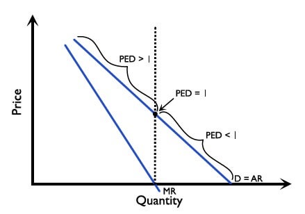
Marginal revenue (MR) is the additional revenue obtained by selling one extra unit of good, and the shape of the MR curve depends on the shape of the demand curve.
Average and marginal revenue with horizontal demand curve
Under perfect competition, firms are price takers and each individual firm faces a horizontal demand curve. In such case the revenue curves are drawn as shown in Figure 2.11.0.3:
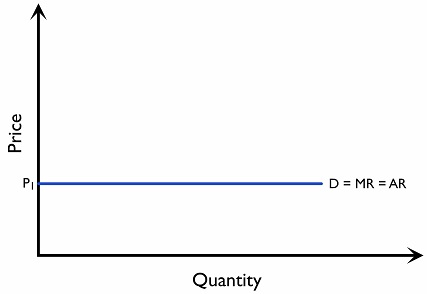
In Figure 2.11.0.3, the price is equal to \(P_1\) at any quantity, and the average revenue curve is same as the demand curve (D=AR). It means that at any quantity, when one additional unit of a good is sold, the marginal revenue gained is \(P_1\). Therefore, the demand curve is the same as the average and marginal revenue curves.
Average and marginal revenue curves with downward sloping demand curve
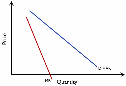
With a downward sloping demand curve, marginal revenue is downward sloping and has a steeper slope than the demand curve. It is because demand = average revenue (AR). As AR decreases, MR has to be smaller than AR to “pull down” the AR, vice versa. (Figure 2.11.0.4)
Profit
Supernormal or abnormal profit is positive economic profit: total revenue exceeds total economic cost, including explicit costs and implicit opportunity costs. It is a return above normal profit.
Economic cost includes both explicit and implicit costs. Implicit cost is the opportunity cost of using the owners’ resources (including time and entrepreneurship) in production, and explicit cost is the type of cost one would find if looking through a firm’s accounting reports.
Normal profit is the minimum return needed to keep the entrepreneur’s resources in their current use. It is an opportunity cost and is included in implicit costs. A firm earns normal profit when total revenue equals total economic cost, so economic profit is zero.
Owners’ resources employed in production could also be used for alternative purposes that can generate revenue. If the foregone revenue is greater than the revenue obtained from production, the owner would be better off by closing down the business and using the resources for alternative purposes. Therefore, to keep the firm in business, revenue needs to at least cover all explicit and implicit costs. This condition is satisfied at the breakeven point, where total revenue equals economic costs, or price (P) =average total cost (ATC). Only normal profit is made.
Calculating costs revenue and profit from data
Cost and revenue data can be used to calculate the return from production and the effect of changing output. Total values refer to the whole output; average values refer to each unit; marginal values refer to a change in output.
| Measure | Calculation |
|---|---|
| Total cost | TC = TFC + TVC |
| Average total cost | AC or ATC = TC ÷ Q |
| Average variable cost | AVC = TVC ÷ Q |
| Marginal cost | MC = ΔTC ÷ ΔQ |
| Total revenue | TR = P × Q |
| Average revenue | AR = TR ÷ Q |
| Marginal revenue | MR = ΔTR ÷ ΔQ |
| Economic profit | π = TR − TC |
Calculating marginal values
To calculate marginal cost, subtract the earlier total cost from the later total cost and divide by the increase in output. Marginal revenue is found in the same way using total revenue. If output rises by more than one unit between rows, the change in the total must be divided by that number of units.
A marginal value calculated between two rows refers to that interval. Average values are calculated using the total and quantity in the same row. Average cost and average revenue are undefined at zero output.
Calculating revenue and profit
For a firm charging the same price on all units sold, AR equals price. If the firm must lower its price to sell more, calculate the new total revenue using the new price and the whole quantity sold. MR then reflects both revenue from additional sales and the reduction in revenue on earlier units.
Subtract economic total cost, including implicit costs, from total revenue to find economic profit. A positive value indicates abnormal profit; zero indicates normal profit; a negative value indicates an economic loss. At a given output, the same calculation can be written as:
Selecting output from a table
Calculate profit at each available output and identify the highest value, comparing it with the result from not producing where relevant. In a smooth model with an interior optimum, profit is maximised where MC = MR and MC rises through MR. In a discrete table, exact equality may not occur. The profit values determine the best available output.
2.11.1 Perfect competition
Market structure describes how the market is organised, in terms of the number of sellers and buyers, the entry and exit barriers, the level of market information available, the degree of price-setting power by firms, and the level of product differentiation. In the following sections, different market structures are analysed and explained.
Perfectly competitive markets do not exist in real life. They were ‘created’ by economists as a benchmark for comparison with other market forms.
Assumptions of the model
- Many buyers and sellers in the market
- Identical/homogeneous goods: There is no difference to the consumer as to where to buy the goods because all goods are the same
- Each firm is a price-taker: each firm takes the prevailing market price as the selling price
- No barriers for entry and exit
- Perfect information: Firms have perfect information about consumers and other firms
Revenue curves
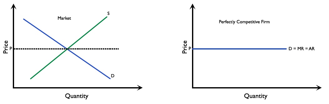
The market price P is determined by the market demand and supply, as shown in the left-hand side graph in Figure 2.11.1. As there are many sellers providing homogeneous products, firms are price takers in perfect competition because there are many sellers, and goods sold are homogeneous. Prices are determined through demand and supply in the market. None of the firms are large enough to influence the market, and firms sell all their stock at the prevailing market price. If they try to charge higher than the market price, buyers would simply buy the item somewhere else. They would not charge lower than the market price because they can sell at the market price. Therefore, each firm has a horizontal (or perfectly elastic) demand curve.
As each additional unit of good generates the same extra revenue, the marginal revenue curve is the same as the demand curve, at price level P.
Cost curves
Firms under perfect competition have short-run cost curves as shown in Figure 2.11.2. Usually only the average total cost curve is drawn.
Perfect competition: Profit maximisation in the short-run and long-run
In this part, the revenue and cost curves are put together to find the profit maximising quantity and output. This part will also show how the market evolves over time in the presence or absence of abnormal profits.
Abnormal profits in the short run
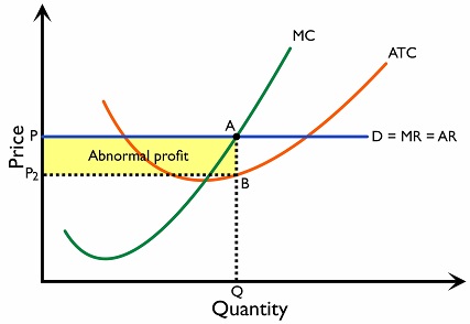
Figure 2.11.3 shows a case where a perfectly competitive firm is making an abnormal profit. First, find the profit maximising quantity and price by noting the point where the marginal cost equals the marginal revenue. It can be seen that at profit maximising quantity Q, the price P is higher than the average total cost (ATC). The firm therefore makes an abnormal profit of \(PP_2BA\), indicated by the shaded area in the graph.
Normal profits in the short run
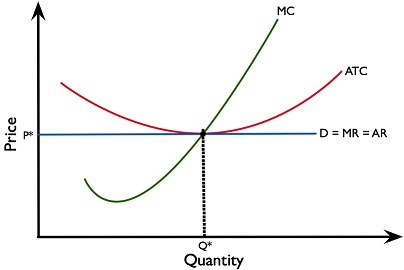
If the price is the same as the average total cost, the firm is making a normal profit. In Figure 2.11.4, the profit maximising price P is the same as the ATC at the profit maximisation level of output. Therefore, the firm’s revenue is the same as its economic costs.
Losses in the short run
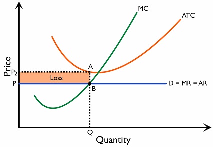
If the price is lower than the average total cost, the firm might be making a loss. In Figure 2.11.5, the profit maximising price \(P\) is below ATC \((P_2)\) at the profit maximisation level of output. Therefore, the firm makes a loss of \(P_2PBA\), denoted by the shaded area in the graph.
Long run
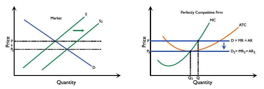
As there are no barriers to entry in a perfectly competitive market, if there were abnormal profits, new firms would enter the market. Consider Figure 2.11.6. Suppose that the market price is originally at price level P. At that level, individual firms would be making an abnormal profit, because P is above the level of ATC.
The presence of abnormal profits attracts new entrants, and as a result, market supply shifts towards the right from \(S\) to \(S_2\). The increase in market supply lowers the market price until \(P_2\), where individual firms can no longer make any abnormal profits. This is the long run equilibrium: at \(P_2\), no firms leave the market, and no firm wishes to enter the market.
The evolution of a perfectly competitive market when firms are making losses is very similar: firms leave the market, reducing market supply. This has the effect of raising prices, and prices go up until they are equal to the level of ATC. In other words, the same outcome is seen on the right-hand graph on Figure 2.11.6.
Efficiency
Allocative efficiency: Price = Marginal cost
For allocative efficiency, the point of interest is whether the goods produced are wanted by society. The demand curve shows the relation between price and quantity, and can also be understood as the curve showing the relation between marginal benefit and quantity. For instance, if P = 10 at Q =2, it must follow that the second unit of the good gives a benefit that is worth of $10; otherwise the consumer would not be willing to pay $10 for the good. The price is the marginal benefit to consumers.
Therefore, price = marginal cost can also be understood as marginal benefit = marginal cost. If marginal benefit > marginal cost, society would be better off producing more product. If marginal benefit < marginal cost, then society would be better off producing less product.
Productive efficiency: Production occurs at minimum ATC.
A firm has productive efficiency if a firm can produce goods using the fewest resources possible. If so, there is no wastage of scarce resources and production can be considered efficient. In the case where production operates at the minimum average total cost (min ATC), the firm is productively efficient.
Evaluating perfectly competitive markets
To evaluate perfectly competitive markets, the followings should be considered:
(1) Allocative efficiency (P = MC)
In the perfectly competitive market, because the demand curve of the firm is always horizontal, the price and marginal revenue always coincide. When a firm maximises its profits at MC = MR, P is always equal to MC in both the short run and long run.
(2) Productive efficiency (production at minimum ATC)
Productive efficiency occurs at the minimum point of the ATC curve. A firm can have P = ATC at another output, so breaking even does not by itself establish productive efficiency. In the standard long-run perfectly competitive equilibrium, P = MR = MC and P = ATC; hence MC = ATC at minimum ATC. Short-run equilibrium need not satisfy this condition.
(3) Presence of economies of scale
Because each perfectly competitive firm is very small, there is no possibility for economies of scale. This is where a perfectly competitive market may compare unfavourably to other market structures in terms of efficiency, because the economies of scale imply a more efficient use of resources.
(4) Presence of research and development (R&D)
In the long run, perfectly competitive firms make no abnormal profit and therefore cannot reinvest in R&D. The quality and variety of goods might not be improved over time.
(5) Distribution of gains between firms and consumers
In a perfectly competitive market, none of the firms have sufficient market power to set the price. In the long run, prices are always driven down to the minimum average total cost level, and consumers are the main beneficiaries in this kind of market structure.
2.11.2 Monopoly
Assumptions of the model
(1) One dominant seller in the market
(2) Firms can sell homogeneous or heterogeneous products
(3) The firm is a price setter
Monopoly holds a significant degree of market power, and can choose to produce a quantity that is most advantageous to it; hence it can also choose the price level.
(4) High barriers to entry
A) Legal barriers
A license might be required for firms to operate business in certain industries. For example, in the television operation business in Hong Kong, operators need to obtain a licence from the government; the prerequisite for application might be very demanding and approval of the license can take a long time. This reduces the number of operators in the market. Patents, trademarks and copyright laws to protect inventions and intellectual property are regarded as legal barriers.
B) Economies of scale
Firms which enjoy economies of scale have a large output level with a lower average production cost. New firms might find it hard to compete in a market via price where an incumbent firm is already enjoying economies of scale and can price down its products to drive out competitors.
C) Branding
If the market has a strong level of brand loyalty, new firms might find it hard to gain market share from incumbent firms. This might deter new firms from entering the market.
Revenue curves
The demand curve of a monopolist is the familiar downward sloping demand curve, as seen in Figure 2.11.8. The MR curve is downward sloping and steeper than the demand curve.
Cost curves
The short run cost curves (Figure 2.11.9) of a monopolist look similar to that of a perfectly competitive firm:
Profit maximisation
To maximise profit, a monopolist chooses to produce the quantity corresponding to the profit maximising condition MC = MR. The market price (P) will then be the price corresponding to the profit maximising quantity (Q) on the demand curve. Figure 2.11.10, 2.11.11 and Figure 2.11.12 show the scenarios where the monopoly is making abnormal profit, normal profit and loss respectively.
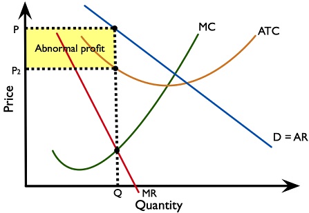
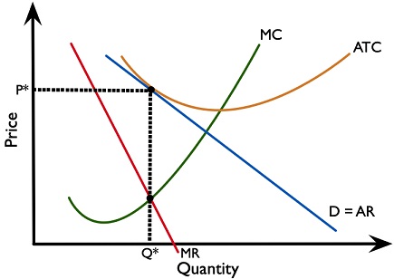
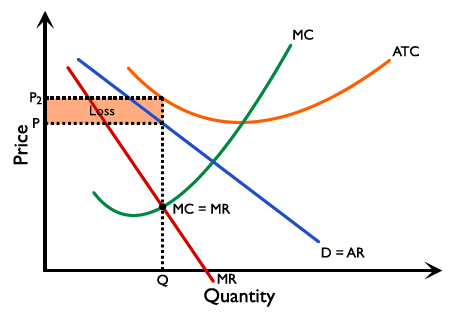
To know if a monopolist is making an abnormal profit or loss, compare the price and the average total cost at the profit-maximising quantity. If P > ATC, then the firm is making an abnormal profit. If P < ATC, then the firm is making a loss. If P = ATC, the firm is only making a normal profit.
Unlike perfectly competitive markets where new firms can enter freely into the market if abnormal profit exists, there are significant barriers to entry in a monopoly. If no outside firm can overcome these barriers to enter the market, the monopoly can keep on making abnormal profit in the long run. In this case, the long run equilibrium is represented by the same graph as that for the short run equilibrium.
Natural monopoly
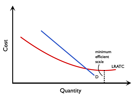
Unlike firms in perfect competition, a monopolist has sufficient scale to take advantage of economies of scale, i.e. where average total cost (ATC) decreases as quantity increases. A natural monopoly exists when an industry can only support one firm with the level of economies of scale available. Industries with high sunk cost that require large levels of output to exploit economies of scale are usually a natural monopoly, e.g. utilities companies. The graph of a natural monopoly is illustrated in Figure 2.11.14. It can be seen that the average total cost is decreasing over a large stretch of quantity, implying that significant economies of scale can be obtained with only one firm in the market.
Monopoly and Efficiency
1) Allocative inefficiency
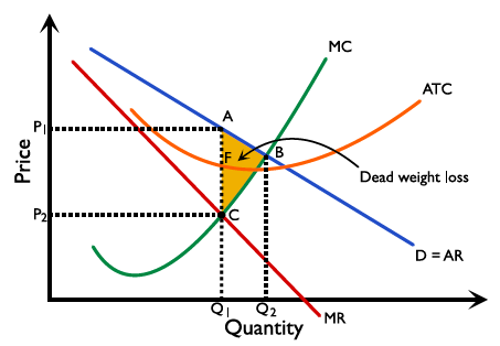
Allocative efficiency occurs at P=MC. In Figure 2.11.15, a profit-maximising monopoly will produce at \(Q_1\), where MC = MR. At \(Q_1\), the price is at \(P_1\) and MC is at \(P_2\). The price is larger than MC and allocative efficiency is not achieved. The society suffers a welfare loss equal to the area ABC.
2) Productive inefficiency
Productive efficiency is not achieved under a monopoly, as the firm will always produce up to MC = MR, but not necessarily operating at the minimum ATC.
Monopoly vs. perfect competition
The comparison between monopoly and perfect competition is summarised below.
| Perfectly competitive firm | Lower price and higher output |
|---|---|
| A Monopolist | Higher price and lower output |
| Perfectly competitive firm | Allocative efficiency Allocative efficiency can be achieved as the firm produces at P = MC. |
|---|---|
| A Monopolist | Allocative inefficiency
Allocative efficiency is not attained as the firm produces at P > MC. |
| Perfectly competitive firm | May not be able to finance research and development (R & D)
Perfectly competitive firms do not make abnormal profit in the long run and lack abundant funds to finance R & D. |
|---|---|
| A Monopolist | Able to finance research and development (R & D)
Monopoly firms are usually bigger in scale with sufficient funds compared to perfect competitive firms. Monopoly firms also enjoy abnormal profit that can be spent on research and development. Society as a whole gains from higher quality products produced. |
| Perfectly competitive firm | Lack incentive to innovate
Firms lack incentive to innovate as it may be copied by other firms in the market. |
|---|---|
| A Monopolist | Incentive to innovate
In order to maintain the abnormal profit, monopoly firms have an incentive to innovate and be more competitive when facing competition from close competitors. |
|
Perfectly competitive firm |
May not be able to enjoy economies of scale
Each perfectly competitive firm takes up a small percentage in the market. It does not enjoy economies of scale. The average production cost may be higher than monopoly firms. |
|---|---|
| A Monopolist | Able to enjoy economies of scale
Monopoly takes up a large percentage of market share in the market. It may be able to enjoy economies of scale and lower production costs. The average production cost may be lower than the productive efficiency point of perfectly competitive firms in the long run. |
Regulation of monopoly power
It is generally accepted that more competition is better to society. Governments have a range of antimonopoly polices to reduce monopoly power.
1) Taxes
Abnormal profit can be taxed away to redistribute income from monopolists to tax payers so as to improve equity between firms and consumers.
2) Privatisation
Many monopolists are formed under legal regulations and some are state-owned. By privatising state-owned firms, they can be split into private firms and encourage competition.
3) Nationalisation
In other cases, the government might choose to nationalise an industry. This is likely to be the case with natural monopolies, where it is difficult to promote competition. For example, many countries have nationalised the railroad industry.
In the 2019 UK general election, the Labour party campaign promised to nationalise various industries including broadband, rail, the postal service, water, and energy. The party’s manifesto promised that these nationalisations would reduce monopoly power and therefore improve the provision of public services and reduce costs for consumers.
In response, many argued that nationalisation would be too expensive; for example, Jefferies, an investment bank, estimated that nationalising the UK’s power utilities alone would cost £124 billion.
However, it may not be the case that re-nationalization of these industries would cost the taxpayer more. For example, the average water bill in 2015 was £396, £113 higher than if water prices had risen in line with inflation since the industry was privatised in 1989. These higher prices under privatisation reflect the fact that private companies pay shareholder dividends and face higher interest rates.
In the UK, the railways are owned by a nationalised company. The right to run trains on the tracks are then allocated by auction to various privately-owned firms. This system aims to maximise the benefits of both nationalisation and competition.
4) Deregulation
Deregulation of the market involves lowering the entry barrier so that more firms can enter the market to compete and reduce monopoly power.
For example, the US Energy Policy Act (1992) aimed to remove obstacles for competition in the market for wholesale electricity in order to encourage firms to enter and achieve some of the benefits of competition.
5) Regulation
Governments can pass laws which restrict the ability of firms to grow through mergers or takeovers.
For example, in the UK, mergers which would result in the new company controlling more than 25% of the market are not allowed.
‘Antitrust’ laws are laws which aim to increase competition in the economy and reduce monopoly power. The three main pieces of antitrust legislation in the United States are the Sherman Act (1890), the Clayton Act (1914), and the Federal Trade Commission Act (1914).
The Sherman Act regulates competition between companies. It prohibits any anti-competitive agreements, and any conduct that monopolises or aims to monopolise the market. It allows entrepreneurs to achieve monopoly status by merit, but prohibits the artificial increase of prices, and any action by such an ‘innocent’ monopolist to artificially preserve their monopoly status.
The Clayton Act adds to the Sherman Act by aiming to stop anticompetitive practices in their infancy. It prohibits price discrimination if it will lessen competition or create a monopoly, mergers if they stand to lessen competition, and any person from being a director of two or more competing corporations if they would violate the antitrust criteria by merging.
The Federal Trade Commission Act established the Federal Trade Commission (FTC). The FTC is an independent agency which aims to enforce antitrust law, and promote consumer protection.
In 2011, the FTC challenged the proposed acquisition of Palmyra Medical Center by the hospital authority that owned Phoebe Putney Memorial Hospital in Georgia, arguing that it would reduce competition. The acquisition nevertheless completed in December 2011. The case later resulted in a 2015 consent order; it is an example of a merger challenge, not a merger successfully blocked in 2011.
6) Fines
Governments sometimes set up regulatory bodies for certain industries, usually industries where there would otherwise be a natural monopoly, to protect the interests of consumers. For example, the UK’s electricity market is regulated by the Office of Gas and Electricity Markets (Ofgem).
Regulatory bodies have different powers to prevent the exertion of monopoly power. One of these is imposing fines for anti-competitive behaviour. For example, in 2019 Ofgem charged Economy Energy, an energy company, a fine of £200,000 for violating the Competition Act 1998.
According to EU competition law, the European Commission (EC) can fine a firm that has engaged in anti-competitive behaviour. These fines are calculated by multiplying the percentage of the company’s annual sales of the product that was concerned in the infringement of the law (up to a maximum of 30%) by the number of years and months that the infringement lasted. Companies that are repeat offenders can face higher fines, while those who had limited involvement might be fined a smaller amount. The fine is capped at 10% of the overall annual revenue of the company.
The fines are intended to deter companies from breaking competition law; they are therefore calculated to punish and to deter, and therefore to change companies’ incentive structure when they consider abusing monopoly power.
For example, in 2018 the EC fined Google €4.34 billion on the grounds that it had imposed illegal restrictions on Android device manufacturers and mobile network operators in order to strengthen its monopoly on internet searches. It did so in particular by requiring manufacturers to pre-install the Chrome browser and Google Search app in order to be able to use the Play Store, and making payments to manufacturers and mobile network operators on the condition that they exclusively pre-installed the Google Search app on their devices.
2.11.3 Monopolistic competition
Assumptions of the model
- Many buyers and sellers in the market
- Heterogeneous/differentiated goods: Firms are selling products with differentiation such as packaging, branding, after-sales services etc.
- Low degree of price setting
- Low barriers for entry and exit
- Imperfect information
Some typical examples are restaurants, fashion stores and bakeries.
Revenue curves
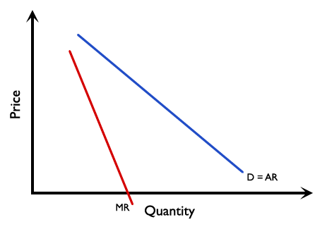
Firms in monopolistic competition sell differentiated products and have a small degree of monopoly power. Therefore, firms face a downward sloping demand curve similar to the monopoly firm as shown in Figure 2.11.16. However, a monopolistically competitive firm faces a more elastic demand curve compared to a monopoly. This is because a monopolistically competitive firm has less market power due to many substitutes available in the market.
Cost curves
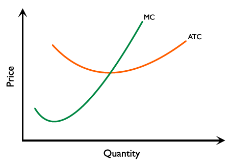
The short run cost curves of monopolistic competition are similar to those of monopoly firms as shown in Figure 2.11.17.
Profit maximisation in the short-run and long-run
Short Run
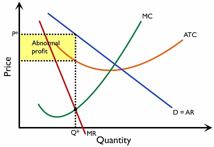
Monopolistic competitive firms shall set prices at the profit maximisation level where MC=MR. In Figure 2.11.18, a monopolistic competitive firm will produce up to Q* and charge a price at P*, enjoying an abnormal profit in the short run.
Losses under monopolistic competition
A monopolistically competitive firm can make an economic loss in the short run. This occurs when average total cost is greater than average revenue at the firm's chosen output.
In Figure 2.11A, the firm produces Q* where MC = MR on the rising section of the MC curve. The price P* is read from the demand curve, D = AR, directly above Q*. Average total cost at this output is AC*, which is greater than P*.
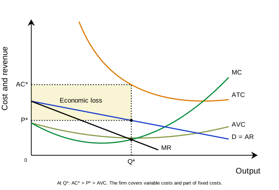
Total cost = AC* × Q*
Economic loss = (AC* − P*) × Q*
The shaded rectangle shows the loss. Producing at MC = MR does not guarantee a profit. In this case it gives the firm the smallest loss from producing.
Short-run production and long-run exit
The firm shown continues producing in the short run because price is above average variable cost at Q*. Revenue covers variable costs and contributes towards fixed costs. Closing immediately would leave the firm with its fixed costs and no revenue. If the best available price–output combination cannot cover variable costs, shutting down would give a smaller loss.
Persistent losses cause some firms to leave the industry in the long run. Consumers then have fewer substitutes, so demand for the remaining firms increases. Under the standard model, exit continues until the remaining firms earn normal profit. At this position, price equals average total cost at the profit-maximising output.
Normal profit includes the opportunity cost of the owner's resources. It does not mean that the owner receives no income.
Long Run
In the long run, the abnormal profit in a monopolistic competition will attract new firms to enter the market and compete with the existing ones, as there is a low entry barrier. The demand for individual firms shall decrease from \(D_1\) to \(D_2\) and the marginal revenue curve will move from \(MR_1\) to \(MR_2\)as shown in Figure 2.11.19.
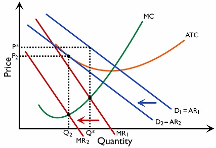
Entry will continue until the abnormal profit of the firm dissipates. Now the firm in monopolistic competition produces at \(Q_2\) and the price is at \(P_2\). The firm earns zero abnormal profit, which means it is only making normal profit.
Non-price competition
In order to maintain profit by differentiating from other competitors, firms will engage in both price and non-price competition.
Price competition refers to a situation where firms compete for sales by the means of lowering price. For example, firms may provide discounts to attract consumers.
Non-price competition refers to a situation where firms compete for sales by means of non-price methods. Firms in the apparel and beauty market often use heavy advertising and packaging to stand out from competitors. Jewel manufacturing firms invest in product development and service quality improvement, to develop unique selling points to maintain product differentiation from other firms.
Monopolistic competition and efficiency
Neither allocative efficiency nor productive efficiency can be achieved by monopolistic competitive firms. In both Figure 2.11.18 and 2.11.19, monopolistic competitive firms are producing at a point where P is larger than MC and it is not necessary for them to operate at the minimum ATC level.
Table 2.11.3 Comparison among monopoly, monopolistic competition and perfect competition
| Perfect competition | Monopoly | Monopolistic competition | |
|---|---|---|---|
| Number of producers | Many | One dominant producer | Many |
| Size of firms | Small | Large | Small to Large
(depends on market power) |
| Economies of scale | Not able to enjoy | Able to enjoy | Some are able to enjoy |
| Short Run | Abnormal profit can be enjoyed | Abnormal profit can be enjoyed | Abnormal profit can be enjoyed |
| Long Run | Only normal profit can be enjoyed | Abnormal profit can be enjoyed | Only normal profit can be enjoyed |
| Market Power | Nil | Large | Limited |
| Allocative efficiency | Achieved | Not achieved | Not achieved |
| Productive efficiency | Achieved | Not necessarily achieved | Not necessarily achieved |
| Ease of entry and exit | No entry barriers | High entry barriers | Low entry barriers |
| Product differentiation | Homogeneous product | Unique product
(when there is only one monopoly in the market) |
Differentiated product |
2.11.4 Oligopoly
Assumptions of the model
1) Few dominant players in the market
2) Firms are interdependent on each other
An action of a single firm will trigger actions by other competitors. If Sony decides to cut the price of the PlayStation console, then it is expected that Microsoft will also cut the price of the Xbox console in order to maintain the market share.
3) Firms sell homogeneous or differentiated products
Oligopolistic firms sometimes produce homogeneous products (such as petrol stations, supermarkets), while some produce differentiated products (such as car manufacturers).
4) High barriers to entry
Concentration Ratio
Calculation of the concentration ratio is useful in determining whether the market structure is an oligopoly.
The concentration ratio is calculated by summing up the market share of the dominant firms. For example, the top 4 supermarkets in the UK take up 80% of the market share. We say that the market is highly concentrated and is an oligopolistic market structure.
Game theory and interdependence
We can use the game theory to illustrate the interdependence of oligopolistic firms. Let us start with the prisoner’s dilemma.
Prisoner’s dilemma
Criminal A and B robbed a bank together and were caught. As there was no actual proof for the crime, the police could only charge them “armed with illegal guns”. However, the police believe that they had committed other serious crimes, so went on questioning them individually. The terms of various responses from the criminals are summarised as follows:
- Both of the criminals admitted committing a serious crime: both are sent to jail for 10 years.
- One admits guilt but the other does not: the one that admitted will be set free and the other one will go to jail for 15 years.
- Both of them do not admit: both are sent to jail for 1 year.
We now put the payoff of different situations in an outcome matrix in Table 2.11.4.
Read each pair as (B, A): the row player’s outcome comes first and the column player’s second. In the prisoner example the entries are years in prison, so a smaller number is better.
| Criminal A | |||
|---|---|---|---|
| Admit | Not Admit | ||
| Criminal B | Admit | (10,10) | (0,15) |
| Not Admit | (15,0) | (1,1) | |
To criminal A, if he admits, the outcome can be 10 or 0 years jail, depending on criminal B’s choice. If criminal A does not admit, the outcome can be 15 or 1 year jail. The best strategy for A is to admit to the crime. It is because admitting makes A better off, regardless of whether B admits or not. Symmetrically, this is the same for criminal B. Ultimately, when they consider others’ action and they both will choose to admit and both are sent to jail for 10 years. However, if they can cooperate and both do not admit guilt, both of them will only be sent to jail for 1 year.
Oligopolistic firms make decisions on pricing strategies similarly. Suppose there are 2 firms and they are considering whether to cut price or not. The scenarios are as follows:
- Both firms cut their price: both firms will lose 10 million from lowering profit.
- One cuts the price and one keeps it unchanged: The firm cutting the price will enjoy an increase in profit by 5 million, while the one keeping it unchanged will suffer a loss of 13 million from losing demand.
- Both firms keep the price unchanged: Both firms will experience no change in the total profit.
We now put the payoff of different situations in an outcome matrix in Table 2.11.4.
The same order applies: (Firm B, Firm A). Each entry is the change in profit, in millions; a larger number is better. For example, (+5, −13) means B gains 5 million while A loses 13 million.
| Firm A | |||
|---|---|---|---|
| Cut price | Leave the price unchanged | ||
| Firm B | Cut price | (-10,-10) | (+5,-13) |
| Leave the price unchanged | (-13,+5) | (0,0) | |
To firm A, if it cuts the price, it will either suffer a loss of 10 million or gain 5 million. If it leaves the price unchanged, it will either suffer a loss of 13 million or keep its profit unchanged. Symmetrically, it is the same for firm B. For both firms, they are both better off if they choose to cut the price after considering the actions of the competitor. Ultimately, they will both choose to cut the price and both suffer a loss of 10 million. However, if they can cooperate, both of them will benefit from maintaining the price and prevent a loss in profit.
The dilemma faced by oligopolistic firms as illustrated above explains that leaving the price unchanged is a better option for both firms. However, there is a risk that one firm might cheat, resulting in a less desirable outcome for another firm. Although there is an incentive for firms to collude and cooperate, firms need to have mechanisms to protect the other from cheating before cooperating.
Open/ Formal Collusion
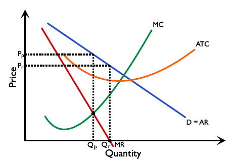
Collusion exists when a small number of firms act together to avoid competition by resorting to agreements to fix prices or outputs. Collusive oligopoly acts like a monopoly. (Refer to Figure 2.11.4.1)
Cartel
A cartel means a group of producers in an industry that join together to regulate supply and fix price. A cartel is usually illegal, as there are competition laws forbidding private cartels in most countries. The Organisation of the Petroleum Exporting Countries (OPEC) is one example of a cartel between oil exporting countries that fix the price and output levels.
Firms in a cartel behave like a monopoly. The goal of a cartel is to limit competition between firms and to maximise joint profit.
Evaluation of the cartel
The price agreed in the cartel is often set high to generate higher profits. This is done through agreements by members to voluntarily reduce output level. There is an incentive for firms to cheat by producing more than the agreed amount of output in the market. If all members cheat and increase their supply, the price level will be pushed down and the cartel will collapse.
The conditions that make cartel structures difficult to maintain
- A large number of member firms; it makes monitoring more difficult
- The member firms hold a small proportion of market share; it is hard to control the market price
- Firms sell differentiated goods; it is hard to set an agreed uniform price
- Differentiated production cost
- Shrinking market size; raises the incentive for firms to cheat in order to survive
Tacit/Informal Collusion
Tacit collusion exists when there is a dominant firm and few smaller competitors in the market. The dominant firm will set a relatively high price to maximise his profit,
and other smaller firms will accept and follow by selling at the high price level.
Non-collusive oligopoly
Non-collusive oligopoly exists when the few dominant firms do not act together to avoid competition by resorting to agreements to fix prices or outputs. A non collusive oligopoly can be represented using a kinked demand curve.
Kinked demand curve and price rigidity
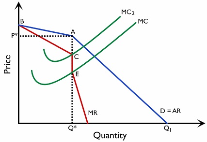
The assumptions behind the kinked demand curve model are that rival firms will follow a price cut of its competitors but not a price rise, and price level is rigid in general.
When the firm sets a price higher than P*, rival firms will not follow the price rise. This lowers the quantity demanded of the firm who raises the price and decreases the total revenue received by the firm. The demand curve portion of AB is relatively elastic as raising the price causes a drop in revenue.
When the firm sets a price lower than P*, rival firms will follow the price cut and this lowers the total revenue of the firm who decreases the price. The demand portion of AC is relatively inelastic as lowering price causes a drop in revenue.
Since the slope of the demand curve portion AB and AQ1 is different, the MR curves drawn therefore have different slopes. A discontinuous MR curve is formed at the kink of the demand curve. The implication is that even if the production cost for the firm increases and pushes the MC curve up to MC2, the profit-maximising output level is still at Q*. The price remains at P*. The low possibility of the MC curve falling out from the region CE explains the existence of price rigidities in an oligopoly.
Non price competition
Oligopolistic firms generally avoid price competition as a price cut will usually be followed by rival firms, leading to a price war. Eventually, all firms will be worse off as firms are no longer producing at the profit maximisation level. Consumers will be better off by enjoying lower price levels. Weaker firms with insufficient funds will be driven out of the market.
Non-price competition is common among oligopolistic firms. Supermarket chains have consumer loyalty programs so that consumers get rewarded for continuous purchases; camera manufacturers often provide after-sales services and extended guarantees etc.
Price competition
Oligopolistic firms could engage in price competition with the objective to drive competitors out of the market. For example, a firm in an oligopoly could lower its price to encourage consumers to buy from it instead of its competitors. The firms’ competitors therefore face a loss in demand, and therefore a reduction in profit. This may force them to leave the market. Once they do, the original firm can raise its price again, to a higher level than was possible before when there were more competitors in the market.